Likelihood, Bayes and Information Theory
Why models minimise cross-entropy: maximum likelihood, priors and MAP, Bayesian updating, entropy, cross-entropy and KL divergence — the statistics hiding inside every loss function.
📄 Illustrated notes · every chapter as a picture · printable
Quick quiz
5 questions to check your understanding.
Go deeper
University-level written lectures in The AI Lecture Hall:
Transcript
Introduction. Why do classifiers minimise cross entropy? Why does squared error appear in regression? Why do we add weight decay? The answers come from two beautiful fields: statistical estimation and information theory. This deep dive connects them to the loss functions you use every day.
Parameters and data. A statistical model is a family of probability distributions controlled by parameters, written p of x given theta. A Gaussian has two parameters, a mean and a standard deviation. A neural network is also a probability model, with millions of parameters. Learning means choosing good values for theta.
Likelihood. The likelihood asks: if the parameters were theta, how probable would the data we actually observed be? For independent data points it is the product of each point’s probability. It uses the same formula as probability, but we read it as a function of the parameters with the data held fixed.
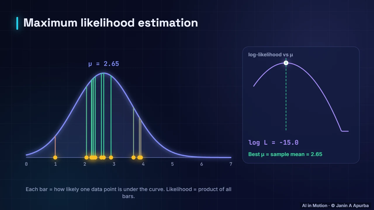
Maximum likelihood. Maximum likelihood estimation picks the parameters that make the data most probable. Watch the Gaussian slide along. Each bar shows how likely one data point is under the current curve. The log likelihood, on the right, peaks exactly at the sample mean, two point six five. That is the maximum likelihood estimate.
Why take logs?. In practice we maximise the log likelihood instead. The logarithm turns a product of many tiny probabilities, which would underflow to zero on a computer, into a sum of manageable numbers. Because the log only increases, the best parameters do not change, and sums are easy to differentiate.
Loss = negative log-likelihood. Flip the sign and average, and you get a loss to minimise: the negative log likelihood. This single idea generates the standard losses. If you assume Gaussian noise around the prediction, it becomes squared error. If the output is a category, it becomes cross entropy.
Pause and think. Pause and think. A model assigns probability point nine to the correct class for one example, and only point one for another. What is the loss for each? Minus the log of point nine is about point one one, a small loss. Minus the log of point one is about two point three: confident mistakes are punished heavily.
The shape of the loss. This curve shows the loss for one example as a function of the probability given to the correct answer. At point nine the loss is tiny. At one half it is about point seven. As the probability approaches zero, the loss shoots up towards infinity, so the model is pushed hard never to be confidently wrong.
Estimators. An estimate computed from data is itself random, because a different sample would give a different answer. Its bias asks whether it is right on average, and its variance asks how much it wobbles. The sample variance divides by n minus one instead of n precisely to remove a small bias.
Bias and variance. The dartboard picture makes this concrete. Low bias and low variance cluster tightly on the bullseye. High bias misses consistently in one direction. High variance scatters widely. The same trade off governs models: simple models tend to be biased, while very flexible ones tend to have high variance.
Priors. Maximum likelihood listens only to the data, which is risky when data is scarce. Bayesian statistics adds a prior: what we believe about the parameters before seeing any data. For example, believing that weights are probably small corresponds to a Gaussian prior centred on zero.
Posterior. Bayes’ theorem combines the two. The posterior, our belief after seeing the data, is proportional to the likelihood times the prior. With little data the prior dominates. With lots of data the likelihood takes over and the prior washes out.
Bayesian updating. Here is Bayesian updating with a coin of unknown bias. We start with a gentle prior centred on one half. As flips arrive, the posterior curve shifts and narrows. After forty flips with twenty eight heads, it concentrates near point seven: more data means more confident beliefs.
Pause and think. Pause and think. A coin lands heads seven times in ten flips. What is the maximum likelihood estimate of its bias? Seven tenths. With a gentle Beta two, two prior, the MAP estimate is eight twelfths, about point six seven, pulled a little towards one half by the prior belief.
MAP estimation. Often we want a single best answer: the peak of the posterior, called the maximum a posteriori, or MAP, estimate. Its loss is the negative log likelihood minus the log prior. With a Gaussian prior on the weights, that extra term is exactly L two regularisation, also known as weight decay.
Priors as regularisers. Different priors give different regularisers. A Gaussian prior gives the L two penalty, a circle, which shrinks all weights a little. A Laplace prior gives the L one penalty, a diamond, whose corners push some weights to exactly zero. Here the L one solution lands on a corner: a sparse model.
Pause and think. Pause and think. You have twenty training examples and ten thousand features. Should you rely on maximum likelihood alone? No. With so little data, maximum likelihood will happily overfit. A prior, in other words regularisation such as L one or L two, is essential, or better still, collect more data.
Information. Now to information theory, founded by Claude Shannon. The information in an outcome is its surprise: minus the log of its probability. A fair coin flip carries one bit. An event with a one in eight chance carries three bits. Something certain carries no information at all.
Entropy. Entropy is the average surprise of a distribution. Four equally likely outcomes give the maximum, two bits. As the distribution becomes peaked, entropy falls: one point eight five bits, then one point three six, and finally only about point two four bits when one outcome is almost certain.
Entropy in ML. Formally, entropy is minus the sum of p log p. It is the minimum average number of bits needed to encode outcomes from that distribution, which is why it underlies compression. Decision trees use it too: they choose splits that reduce entropy the most, called information gain.
Information gain. Here a decision tree splits the data. A good split creates groups that are purer, each dominated by one class, so the entropy after the split is lower. The reduction in entropy is the information gain, and the tree greedily picks the split with the largest gain.
Cross-entropy and KL. Now suppose the truth is P, in blue, but our model predicts Q, in pink. Cross entropy measures the average surprise when outcomes come from P but we encode them using Q. It starts at two point six eight bits, well above the entropy of P, one point six five. The gap is the KL divergence.
The key identity. This identity is the punchline. Cross entropy equals the entropy of the truth plus the KL divergence. The entropy of the data is fixed, so minimising cross entropy is exactly minimising the KL divergence, pulling the model’s distribution towards the true one. By the end here it is only point zero one five bits.
Cross-entropy in LLMs. Language models are trained with exactly this loss. At every position the model predicts a distribution over the next token, and the loss is minus the log probability of the actual next token. Averaged over a sentence, it is the cross entropy, and its exponential is called perplexity.
Pause and think. Pause and think. Is the KL divergence symmetric? Is KL of P given Q the same as KL of Q given P? No. One direction heavily penalises the model for missing outcomes the truth considers likely, the other penalises it for putting probability where the truth has little. They generally differ.
Perplexity. Language model quality is often reported as perplexity, the exponential of the cross entropy. It has a lovely interpretation: the effective number of equally likely words the model is choosing between at each step. A perplexity of ten means the model is as uncertain as if it were picking among ten words.
Mutual information. One more quantity: mutual information, how much knowing one variable reduces our uncertainty about another. It is zero exactly when the two are independent. It is used to rank features, and contrastive methods like CLIP can be understood as maximising a bound on the mutual information between images and captions.
Where KL appears. KL divergence appears across machine learning. It is inside every cross entropy loss. It keeps the latent codes of variational autoencoders tidy. It stops models tuned with human feedback from drifting too far from the original. It drives knowledge distillation, and related scores monitor data drift in production.
In code. In code, these are one liners. With the truth P and a poor model Q, the entropy is one point six five bits, the cross entropy two point six eight, and the KL divergence, their difference, is about one point zero four bits. Deep learning libraries compute the same thing, usually with natural logs.
Putting it together. Putting it all together: one idea explains many losses. Squared error is the negative log likelihood under Gaussian noise. Cross entropy is the negative log likelihood of categories. Weight decay is a Gaussian prior, and the L one penalty is a Laplace prior that encourages sparsity.
Recap. To recap. Maximum likelihood picks the parameters that make the observed data most probable, and minimising negative log likelihood gives the standard losses. Priors combine with the likelihood into a posterior, and MAP estimation adds regularisation. Entropy is average surprise, and cross entropy is entropy plus KL divergence.