Probability and Distributions for ML
Random variables, expectation and variance, the Bernoulli, binomial and normal distributions, the central limit theorem, Monte Carlo methods and Markov chains — with live simulations.
📄 Illustrated notes · every chapter as a picture · printable
Quick quiz
5 questions to check your understanding.
Go deeper
University-level written lectures in The AI Lecture Hall:
Transcript
Introduction. Machine learning is about making good decisions under uncertainty. Data is noisy, labels are imperfect, and predictions are never certain. Probability is the language for all of this. In this deep dive we build the core ideas and watch them come alive in simulations.
Probability. A probability is a number between zero and one measuring how likely something is. Zero means impossible and one means certain, and the probabilities of all possible outcomes add up to one. A spam filter that outputs point nine seven is saying: I am very confident this email is spam.
Random variables. A random variable is a quantity whose value depends on chance, like the result of a die roll or tomorrow’s temperature. Its distribution tells us which values are possible and how likely each one is. Discrete variables take separate values; continuous ones take any value in a range.
Conditional probability. Conditional probability is the probability of A once we know B has happened. It equals the probability of both, divided by the probability of B. Almost every classifier outputs a conditional probability: the probability of a label, given the input.
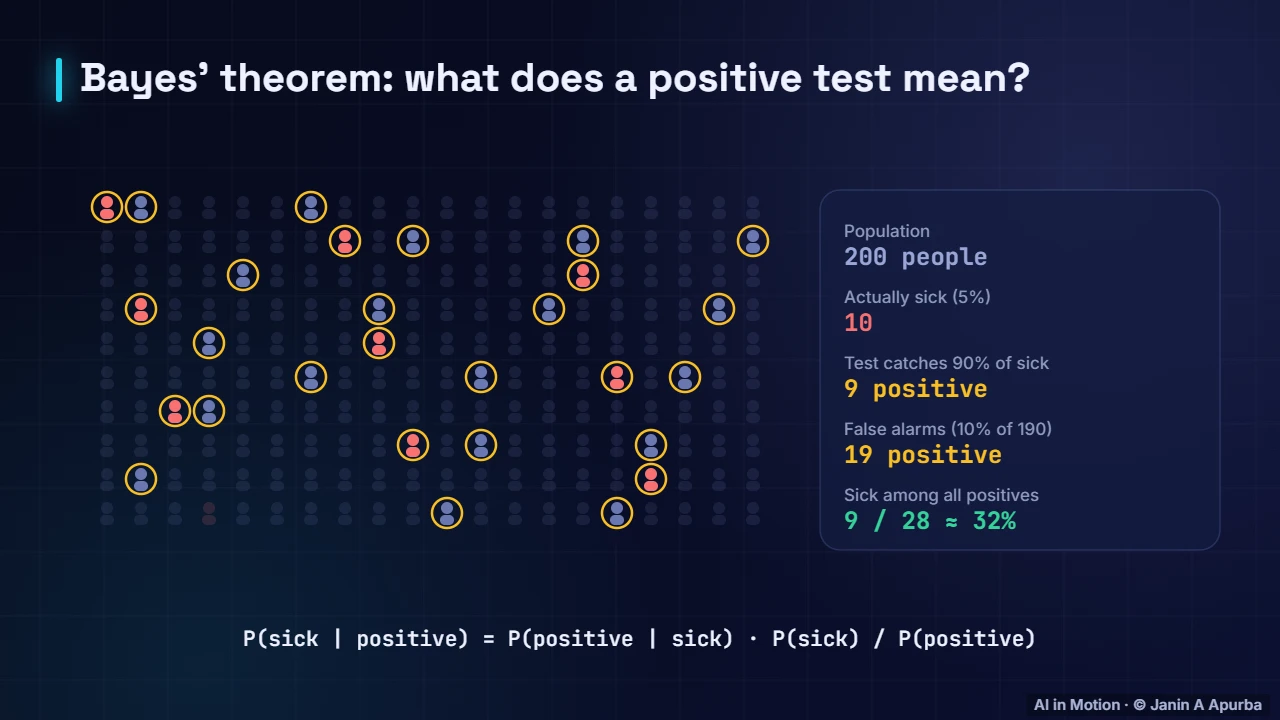
Bayes’ theorem. Bayes’ theorem lets us flip a conditional probability around. Here a disease affects one percent of people, and a test is quite accurate. Yet among everyone who tests positive, most are actually healthy, because healthy people vastly outnumber sick ones. The prior matters enormously.
Pause and think. Pause and think. A test is ninety nine percent accurate, but the condition affects only one person in ten thousand. You test positive. Is it likely you have it? Probably not. In ten thousand people there is about one true positive but around a hundred false positives, so the chance is about one percent.
Bayes in evaluation. Conditional probability is built into how we evaluate classifiers. Precision is the probability that an example really is positive, given that the model predicted positive. Recall is the probability of a positive prediction, given that the example really is positive. Mixing them up is the same mistake as mixing up conditional probabilities.
Expectation. The expected value is the probability weighted average of a random variable, its long run average. For a fair die it is three and a half, even though you can never roll three and a half. Training a model minimises the expected loss over the data distribution.
Variance. Variance measures spread: the average squared distance from the mean. Its square root, the standard deviation, is in the original units. A single die roll has a standard deviation of about one point seven one. High variance means individual outcomes are unpredictable.
Covariance and correlation. Covariance measures whether two variables move together: positive when they rise and fall together, negative when one rises as the other falls. Correlation rescales covariance to lie between minus one and one. Covariance matrices are exactly what PCA decomposes into eigenvectors.
Pause and think. Pause and think. Across a year, ice cream sales and drowning incidents are strongly correlated. Does eating ice cream cause drowning? Of course not. A hidden common cause, hot weather, drives both. Correlation alone never proves causation, and models that learn correlations can be fooled in the same way.
A family of distributions. A handful of distributions cover most of machine learning. The Bernoulli models a single yes or no event. The uniform treats every value in a range equally. The normal, or Gaussian, describes sums of many small effects. The exponential describes waiting times between random events.
The binomial. Repeat a Bernoulli trial n times and count the successes, and you get the binomial distribution. With ten fair coin flips, five heads is most likely. Shift the success probability to point two and the peak moves to two. Its mean is n times p and its variance is n p times one minus p.
The Poisson distribution. Another useful distribution is the Poisson, which counts independent events in a fixed interval, like requests per second arriving at a model server. It has a single parameter, the average rate lambda, which is both its mean and its variance. Engineers use it to plan how many servers to run.
The normal distribution. The normal distribution is the famous bell curve. Its mean, mu, sets the centre, and its standard deviation, sigma, sets the width. Increasing sigma spreads it out and flattens it, because the total area under the curve must always equal one.
The 68–95–99.7 rule. For any normal distribution, about sixty eight percent of values fall within one standard deviation of the mean, ninety five percent within two, and ninety nine point seven percent within three. Values beyond three standard deviations are rare, which makes this a common first rule for spotting outliers.
Pause and think. Pause and think. Exam scores are normally distributed with mean seventy and standard deviation ten. Roughly what fraction scored above ninety? Ninety is two standard deviations above the mean. Ninety five percent lie within two standard deviations, so five percent are in the two tails, and half of that, two and a half percent, is above ninety.
Sampling. Now let us draw random samples from a standard normal and build a histogram. With only ten samples the shape is ragged. As the number grows to thousands, the histogram fills in the true curve, and the sample mean and standard deviation settle close to zero and one.
The law of large numbers. That settling down is the law of large numbers: the average of many independent samples converges to the expected value. It is why larger test sets give more reliable accuracy estimates, and why averaging gradients over a mini batch gives a useful estimate of the true gradient.
The central limit theorem. The central limit theorem is even more surprising. Roll one die and the results are flat, uniform. Average two dice and a peak appears. Average five, then thirty, and a near perfect bell curve emerges, with a spread that shrinks like one over the square root of the number of dice: from one point seven down to about point three.
Standard error. The spread of an average is called the standard error: sigma divided by the square root of n. This square root has a practical sting. To halve the uncertainty of a measurement, such as a model’s accuracy, you need four times as much data.
Monte Carlo methods. Randomness can also compute things. Scatter random points in a square and count how many land inside the quarter circle. Four times that fraction estimates pi. With three thousand points we get about three point one eight, and the error shrinks like one over the square root of the number of points.
Monte Carlo in ML. This idea, estimating an expectation by averaging random samples, is called Monte Carlo estimation. It is everywhere in machine learning. Stochastic gradient descent estimates the true gradient from a random batch, and reinforcement learning estimates the value of a state by averaging sampled returns.
Randomness inside training. Probability is not only for describing data; we also inject randomness on purpose. Dropout switches each neuron off with some probability during training, a Bernoulli coin flip per neuron. This stops the network from relying on any single unit and acts as a powerful regulariser.
Markov chains. A Markov chain is a random process where the next state depends only on the current one. In this weather model, a sunny day is followed by sunshine seventy percent of the time. Run it for many steps and the time spent in each state converges to a fixed long run distribution.
Why Markov chains matter. The key assumption is the Markov property: the future depends only on the present, not on how we got here. It underpins Markov chain Monte Carlo sampling, hidden Markov models for speech, Google’s PageRank, and Markov decision processes, the foundation of reinforcement learning.
Independence. Two events are independent when knowing one tells you nothing about the other, so their joint probability is the product of their separate probabilities. Much of machine learning assumes the data is independent and identically distributed, and many real failures happen when that assumption breaks.
Probabilities from a network. Neural networks produce probabilities with the softmax function, which turns any list of scores into positive numbers that sum to one. A temperature setting sharpens or flattens the distribution, which is exactly how language models control how adventurous their word choices are.
In code. In code, NumPy’s random generator makes these experiments easy. Draw five thousand normal samples and the mean and standard deviation come out close to zero and one. About sixty eight percent fall within one standard deviation, and averages of thirty dice have a spread of about point three one.
Pitfalls. Beware of common pitfalls. Base rate neglect ignores how rare a class is. Confusing the probability of A given B with B given A is a classic error. Assuming independence fails for time series and grouped data. And small samples have large standard errors, so their averages can mislead.
Recap. To recap. Probabilities lie between zero and one and sum to one. Bayes’ theorem reminds us that priors matter. Expectation is the long run average and variance is the spread. For a normal distribution, sixty eight, ninety five and ninety nine point seven percent lie within one, two and three sigma. And averages converge and become normal.