Search and Problem Solving: A Deep Dive
How AI systems find solutions: state spaces, breadth-first, depth-first, uniform-cost, greedy and A* search, admissible heuristics, local search, simulated annealing, genetic algorithms and constraint satisfaction.
📄 Illustrated notes · every chapter as a picture · printable
Quick quiz
5 questions to check your understanding.
Go deeper
University-level written lectures in The AI Lecture Hall:
Transcript
Introduction. Finding a route on a map, solving a puzzle, scheduling exams, planning a robot’s moves: all of these are search problems. Search is one of the oldest and most useful ideas in artificial intelligence. In this deep dive we build it up from first principles to the algorithms used in practice.
What is a search problem?. Every search problem has the same ingredients: a set of states, a starting state, the actions available in each state, a transition model saying where each action leads, a test for whether we have reached the goal, and a cost for each path. Route planning is the classic example.
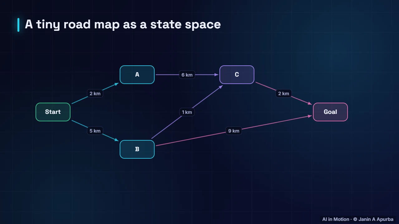
A state space. Here is a tiny road map as a state space. Each town is a state and each road an action with a cost. From Start, the road to A looks shortest, but the cheapest complete route is Start, B, C, Goal, costing eight kilometres. Choosing well means looking beyond the first step.
Frontier and explored set. All search algorithms share one loop. They keep a frontier of states that have been discovered but not yet expanded, and an explored set of states already handled, so no work is repeated. The only thing that changes between algorithms is the order in which the frontier is expanded.
Two families. Search algorithms come in two families. Uninformed, or blind, search knows only the problem definition and explores systematically, like breadth first and depth first search. Informed search also uses a heuristic, an estimate of how far each state is from the goal, to focus on promising directions.
Breadth-first search. Breadth first search explores in ripples. It visits every cell one step away, then every cell two steps away, and so on, using a queue. Because it expands by distance, the first time it reaches the goal it has found a shortest path, here thirty seven moves.
BFS properties. Breadth first search is complete: if a solution exists, it will find it. It is optimal when every step costs the same. But its time and memory grow as the branching factor to the power of the depth, because it stores the whole frontier. That exponential growth is its weakness.
Exponential growth. How bad is exponential growth? With ten choices per state, depth ten already has ten billion nodes. At about a hundred bytes each, storing them needs a terabyte of memory. For deeper problems, breadth first search runs out of memory long before it runs out of time.
Depth-first search. Depth first search dives down one path as far as it can, and only backtracks at dead ends. It uses a stack instead of a queue. It needs very little memory, but look at the path it found: seventy three moves, nearly twice the shortest route.
BFS vs DFS. Side by side, breadth first uses a queue, is complete and optimal for equal costs, but needs huge memory. Depth first uses a stack, needs little memory, but can get lost in infinite spaces and returns poor paths. Iterative deepening combines their strengths by running depth limited searches of growing depth.
Uniform-cost search. When actions have different costs, breadth first search is no longer optimal. Uniform cost search, essentially Dijkstra’s algorithm, always expands the state with the lowest total cost so far, written g of n. On our road map it correctly finds the eight kilometre route through B and C.
Pause and think. Pause and think. On our road map, why would breadth first search, which counts roads rather than kilometres, choose a worse route? It minimises the number of steps, so it prefers Start, B, Goal: only two roads, but fourteen kilometres, instead of the eight kilometre route with three roads.
Heuristics. Informed search adds a heuristic, h of n: a quick estimate of the remaining cost from a state to the goal, based on knowledge of the domain. On a map, the straight line distance to the destination is a natural heuristic. A good heuristic tells the search where to look first.
Greedy best-first. Greedy best first search always expands the state that looks closest to the goal, using only the heuristic. On this maze it gets lucky and finds a route quickly. On other mazes it can walk into long detours, because it completely ignores the cost already paid to get somewhere.
The A* idea. A star combines both ideas. It scores each state with f equals g plus h: the cost already paid plus the estimated cost still to go. That is an estimate of the total cost of the best solution through that state. A star always expands the state with the smallest f.
A* in action. Here is A star on the same maze. Watch the numbers at the top: f equals g plus h for the current cell. Instead of spreading evenly like breadth first search, it leans towards the goal, and only explores detours when walls force it to. It still finds a shortest path.
Admissibility. A star’s guarantee depends on the heuristic. It must be admissible, never overestimating the true remaining cost, and ideally consistent, never dropping by more than the cost of a step. With such a heuristic, A star is guaranteed to return an optimal solution while exploring far fewer states than blind search.
Pause and think. Pause and think. Is straight line distance admissible for driving distance? Yes: no road can be shorter than a straight line. What about twice the straight line distance? It can overestimate, so it is not admissible. A star may then search faster but return a route that is not the best.
Grid heuristics. On grid maps, the Manhattan distance, the sum of horizontal and vertical gaps, is admissible when moves are only up, down, left and right. Euclidean distance suits free movement. And a heuristic of zero is always admissible, but then A star gets no guidance and becomes uniform cost search.
Better heuristics. Among admissible heuristics, higher is better. If one heuristic is always at least as large as another, and both are admissible, A star with the larger one never expands more states. In the eight puzzle, summing each tile’s Manhattan distance beats simply counting misplaced tiles, often by a huge margin.
A* in code. A star fits in about a dozen lines of Python. A priority queue, ordered by f, holds the frontier. We repeatedly pop the most promising state, stop when it is the goal, and otherwise update each neighbour whenever we find a cheaper path to it, pushing it back with its new f value.
Local search. Sometimes the path does not matter, only the final answer: a good timetable, a chip layout, or the weights of a neural network. Local search keeps just one or a few candidate solutions and improves them step by step, using very little memory even for enormous problems.
Hill climbing. Imagine every possible solution as a point on a landscape, where height means quality. Hill climbing looks at its neighbours and steps to whichever is higher. It climbs quickly, but here it gets stuck on a small local peak, even though a much higher peak exists further away.
Escaping local optima. Simple fixes help. Random restart hill climbing runs the climb from many random starting points and keeps the best result. With enough restarts, one of them begins at the foot of the highest hill. Stochastic hill climbing chooses randomly among uphill moves instead of always the steepest one.
Simulated annealing. Simulated annealing borrows an idea from metalworking. At first the temperature is high, and it often accepts worse moves, jumping around the landscape. As it cools, it becomes pickier. Here it escapes the local peak and settles on the global maximum. Because it uses randomness, it usually escapes, though not on every run.
The acceptance rule. The acceptance rule is elegant. A better move is always taken. A worse move, with a loss of delta E, is accepted with probability e to the delta E over T. When the temperature T is high, even bad moves are often accepted. As T falls, the search becomes almost purely uphill.
Pause and think. Pause and think. A move makes things worse by two. What is the chance of accepting it when the temperature is ten, and when it is one half? At ten, e to the minus point two is about point eight two. At one half, e to the minus four is only about point zero two.
Genetic algorithms. Genetic algorithms search with a whole population. Here each individual is a string of sixteen bits and fitness counts the ones. Selection favours fitter individuals, crossover mixes parents, and mutation flips random bits to keep diversity. Generation by generation, the population evolves towards the perfect string.
Constraint satisfaction. Many practical problems are constraint satisfaction problems: variables, each with a set of possible values, and constraints that must all hold. Sudoku is one: eighty one cells, digits one to nine, and no repeats in any row, column or box. Exam timetabling and map colouring are others.
Solving a CSP. CSP solvers combine backtracking with propagation. Pick the variable with the fewest remaining legal values, try a value, then remove values that have become impossible for neighbouring variables. If some variable is left with no options, backtrack and try another value. Good heuristics make huge puzzles solvable in moments.
Choosing an algorithm. To choose an algorithm: for equal step costs in modest spaces, use breadth first search or iterative deepening. For varying costs, use uniform cost search. With a good admissible heuristic, use A star. When only the final state matters, use local search, and for constraints, use backtracking with propagation.
Where search runs today. Search runs everywhere today. Navigation apps use A star variants over road networks with millions of junctions. Video games run pathfinding for every character, every frame. Robots plan motions around obstacles, and logistics companies use local search to route vehicles, schedule staff and pack containers.
Recap. To recap. A search problem is defined by states, actions, transitions, a goal and costs. Breadth first search finds shortest paths but uses lots of memory, while depth first search is frugal but not optimal. A star adds a heuristic, stays optimal if it is admissible, and local search and CSP solvers tackle huge problems.