Evaluating Machine Learning Models: A Deep Dive
How to know whether a model is really good: train/validation/test splits, cross-validation, confusion matrices, precision, recall and F1, ROC and PR curves, calibration, regression metrics, bias–variance, learning curves and leakage.
📄 Illustrated notes · every chapter as a picture · printable
Quick quiz
5 questions to check your understanding.
Go deeper
University-level written lectures in The AI Lecture Hall:
Transcript
Introduction. Training a model is only half the job. The other half is honestly measuring how well it will work on data it has never seen. Evaluation is where many projects go wrong, with impressive numbers that collapse in the real world. This deep dive shows how to evaluate models properly.
Generalisation. The goal of machine learning is generalisation: performing well on new data, not just on the examples used for training. It is the difference between a student who memorised last year’s exam and one who understands the subject. Training accuracy alone tells you almost nothing.
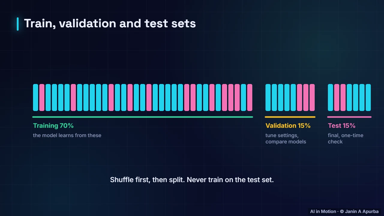
Train, validation, test. The first step is splitting. Shuffle the data so every part is representative, then split it: around seventy percent for training, fifteen percent for validation to tune settings and choose models, and fifteen percent for a final test that we look at only once, at the very end.
Why a separate test set?. Why keep a test set that you look at only once? Every decision made using a dataset, such as picking the best of fifty models, quietly tunes to that data. If you choose using the test set, its score becomes optimistic. The validation set absorbs those decisions, keeping the test set honest.
Cross-validation. With small datasets, one split can be lucky or unlucky. Five fold cross validation splits the data into five parts. Each round trains on four and validates on the fifth, until every part has been the validation set once. Here the five scores average point eight four eight, with a spread showing the uncertainty.
Pause and think. Pause and think. You are forecasting daily electricity demand. Why is ordinary shuffled cross validation a mistake? It lets the model train on days that come after the days it is tested on, peeking into the future. Use time series splits that always train on the past and validate on a later period.
Stratified and grouped splits. Two refinements matter. Stratified folds keep the same class proportions in every fold, which is vital when one class is rare. Grouped folds keep all records from the same person, patient or device together, so the model cannot score well simply by recognising individuals it has already seen.
The confusion matrix. For classification, start with the confusion matrix. We test a spam filter on one hundred emails. Forty two spam emails are caught: true positives. Eight real emails are wrongly marked as spam: false positives. Six spam emails slip through: false negatives. And forty four real emails are correctly left alone.
Precision and recall. Two numbers summarise the positive class. Precision is true positives divided by everything we flagged: how trustworthy the alarms are. Recall is true positives divided by all real positives: how many real cases we caught. Improving one usually costs some of the other.
Compute them. Let us compute them. With forty two true positives, eight false positives, six false negatives and forty four true negatives, precision is forty two out of fifty, eighty four percent. Recall is forty two out of forty eight, eighty seven and a half percent. Accuracy is eighty six out of a hundred.
F1 score. The F1 score combines precision and recall with a harmonic mean, which is high only when both are high. For our filter it is about point eight six. A model with perfect precision but only ten percent recall scores a poor point one eight, exposing the imbalance that an average would hide.
The accuracy paradox. Accuracy can be badly misleading on imbalanced data. If only one percent of transactions are fraudulent, a model that always says not fraud is ninety nine percent accurate, yet it catches no fraud at all. For rare positive classes, look at precision, recall and the metrics that follow.
Pause and think. Pause and think. A cancer screening model has ninety five percent precision but only forty percent recall. Is that acceptable? Probably not: it misses sixty percent of cancers. Screening usually favours high recall, accepting more false alarms that follow up tests can clear.
Many classes. With more than two classes, compute precision and recall for each class and then average. Macro averaging gives every class equal weight, so poor performance on a rare class shows up clearly. Micro averaging gives every example equal weight, so the biggest classes dominate the result.
Pause and think. Pause and think. A three class model scores F1 of point nine five, point nine four and point one on its classes, and the last class is only two percent of the data. Which average reveals the problem? The macro average, about point six six, while the micro average stays above point nine.
Thresholds and ROC. Most classifiers output a score, and a threshold turns it into a decision. Move the threshold left and recall rises but precision falls. Move it right and the opposite happens. Tracing every threshold draws the ROC curve, and the area under it, the AUC, is about point nine four here.
ROC and AUC. The ROC curve plots the true positive rate against the false positive rate for every threshold. Its area, the AUC, has a lovely meaning: the probability that a randomly chosen positive example scores higher than a randomly chosen negative one. Point five is random guessing, and one is perfect ranking.
Precision–recall curves. When positives are rare, the precision recall curve is often more informative than ROC. Because negatives are so numerous, the false positive rate can look tiny even when false alarms swamp the real cases. Precision exposes that directly. Average precision summarises the curve in one number.
Calibration. Ranking is not everything. Calibration asks whether predicted probabilities can be taken at face value: among all cases scored at eighty percent, about eighty percent should turn out positive. Calibrated probabilities matter whenever decisions weigh costs and risks, and they can be fixed after training.
Calibration curve. A reliability diagram checks calibration. The dashed diagonal is perfect. This over confident model predicts extreme probabilities: when it says ninety percent, positives actually occur only about seventy four percent of the time. Deep networks are often over confident, and simple post processing can repair this.
Regression metrics. Regression has its own metrics. Mean absolute error is robust and in the target’s units. Mean squared error and its square root punish large errors heavily. R squared is the share of variance explained. Percentage errors are intuitive but break down when actual values are close to zero.
Pause and think. Pause and think. You predict delivery times, and occasional huge delays really upset customers. Should you optimise mean absolute error or root mean squared error? Root mean squared error, because squaring makes large misses count far more. Mean absolute error treats every minute of error equally.
Underfitting and overfitting. Now the classic trade off. The same data, three models. A straight line underfits, with training error one point five three. A gentle curve fits well. A degree nine polynomial passes through every point with zero training error, but on validation points it is the worst, at two point three. Only validation reveals the truth.
Bias and variance. Think of darts. High bias means consistently aiming off centre, like a model that is too simple to capture the pattern. High variance means throws scattered everywhere, like a model that changes wildly with small changes in its training data. Good models keep both low.
Spotting overfitting. Learning curves reveal overfitting during training. Training loss keeps falling, but validation loss stops improving and starts to rise. The widening gap means the model is memorising. Early stopping keeps the model from the best point, and regularisation or more data narrows the gap.
A healthy curve. When both curves fall together and stay close, the model is genuinely learning rather than memorising. If both stay high, the model is underfitting: it needs more capacity, better features or longer training, rather than more regularisation.
Leakage. The silent killer of evaluations is leakage: information that would not be available at prediction time sneaks into training. Fitting a scaler on the whole dataset, using a feature recorded after the outcome, or having duplicate rows in both training and test sets all make scores look far better than reality.
Baselines. Always compare against a baseline: predicting the majority class, the average, yesterday’s value, or a simple linear model. A ninety two percent accurate model sounds impressive until you learn that always predicting the majority class gives ninety one percent.
Uncertainty in metrics. Every metric computed on a finite test set is itself uncertain. With only one hundred test emails, eighty six percent accuracy could easily be seventy nine or ninety three. Bootstrapping the test set, or using the spread across cross validation folds, gives a confidence interval, and small improvements may be pure noise.
In code. In scikit learn, put preprocessing and the model in one pipeline, so the scaler is re fitted inside every fold and no information leaks. Use stratified folds, request several metrics at once, and report the mean and spread of each across the folds.
Which metric when?. Choose metrics to match the situation. Balanced classes with equal costs suit accuracy and F1. Rare positives need precision, recall and precision recall curves. ROC AUC measures ranking. Probability based decisions need calibration and log loss, and regression chooses between RMSE and MAE by how much big misses matter.
Recap. To recap. Split your data and touch the test set only once. Cross validate with folds that match the problem. From the confusion matrix, derive precision, recall, F1 and curves. Check calibration, pick the right regression metric, watch learning curves, avoid leakage and always beat a baseline.