Gradient Descent and Optimisation: A Deep Dive
Everything about how models are fitted: loss functions, learning rates, batch vs stochastic gradient descent, momentum, Adam and AdamW, schedules, conditioning and feature scaling, saddle points and practical tuning.
📄 Illustrated notes · every chapter as a picture · printable
Quick quiz
5 questions to check your understanding.
Go deeper
University-level written lectures in The AI Lecture Hall:
Transcript
Introduction. Almost every model you will train, from linear regression to a giant neural network, is fitted by some form of gradient descent. In this deep dive we take the algorithm apart: the loss it minimises, the learning rate, stochastic mini batches, momentum, Adam, schedules and the practical tricks that make training work.
Learning as optimisation. Training a model is an optimisation problem. We pick a loss function that measures how wrong the predictions are, and search for the parameters that make it as small as possible. For linear regression, that means finding the slope and intercept with the smallest squared error.
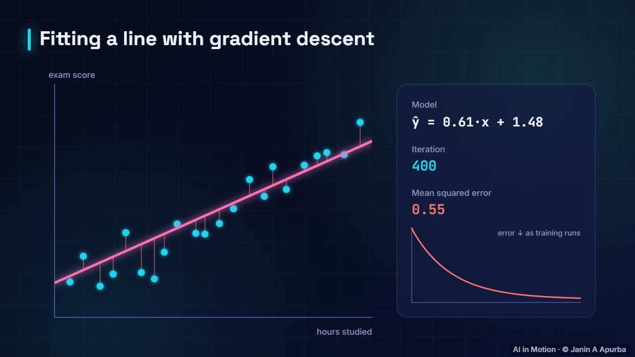
Fitting a line. Here is the process on a simple dataset of study hours and exam scores. The model starts with a bad line and adjusts itself step by step until the line fits the data well. The red lines are the residuals, the errors that the loss adds up. Each step makes them smaller.
The loss. For regression, the usual loss is the mean squared error: the average of the squared gaps between real values and predictions. Squaring punishes large errors heavily and turns the loss into a smooth bowl shaped surface, which is exactly what gradient descent likes.
Walking downhill. Here is gradient descent on one weight. We measure the slope of the loss, the dashed line, and step the opposite way. Where the curve is steep, the steps are big. Near the bottom, the slope flattens and the steps shrink automatically, so the weight settles at the minimum, five point five.
The update rule. The update rule is one line: subtract the learning rate times the gradient. The gradient points uphill, so we step the opposite way. The learning rate, eta, is the single most important setting in training, as the next two examples show.
Too small. With a learning rate that is too small, every step is tiny. After fourteen steps, the weight has only crawled to about two point six, far from the minimum at five point five. Training would take forever, wasting time and compute.
Too large. With a learning rate that is too large, each step overshoots the valley. The weight bounces from one side to the other and never settles, and a little larger still, the loss would explode. There is a sweet spot in between.
Pause and think. Pause and think. Your training loss jumps up and down wildly and then becomes not a number. Which setting should you change first? Lower the learning rate, often by a factor of three to ten. Divergence is the classic sign of steps that are too large, and gradient clipping can also help.
Finding a learning rate. How do you find a good learning rate? Try values on a logarithmic scale, such as one, point three, point one, point zero three, and so on, and pick the largest that trains stably. A learning rate range test raises the rate steadily during one short run and watches where the loss starts to blow up.
Full batch vs stochastic. Real models have many weights, so the loss is a surface. Plain gradient descent uses the whole dataset for every step. Stochastic gradient descent, or SGD, uses a small random mini batch instead. Each step is noisier, as the wobbly amber path shows, but far cheaper, so we can take many more steps.
Batch sizes. There are three variants. Batch gradient descent uses the entire dataset per step: exact but slow. Pure stochastic gradient descent uses a single example: very noisy and inefficient on hardware. Mini batch gradient descent, with somewhere between thirty two and a few thousand examples, is the practical default.
Pause and think. Pause and think. Is the noise in stochastic gradient descent only a nuisance? No. It makes each step cheap, and the randomness can help the optimiser escape saddle points and sharp, narrow minima. Solutions in wide, flat valleys often generalise better to new data.
Momentum. Momentum makes gradient descent behave like a heavy ball rolling downhill. Instead of stepping only by the current gradient, it keeps a running velocity that accumulates past gradients. Consistent directions speed up, while zig zags across a narrow valley cancel out. A typical momentum coefficient is point nine.
Momentum update. In symbols, the velocity is beta times the old velocity plus the new gradient, and the parameters move along the velocity. Gradient components that point the same way step after step add up, while components that flip back and forth cancel out.
Optimisers compared. Here three optimisers race down the same narrow valley. Plain gradient descent zig zags from side to side. Adam adapts its step size for each direction and heads almost straight in. Momentum builds up speed along the valley, and by the end it is closest to the minimum.
Adam. Adam, introduced in 2014, combines momentum with per parameter step sizes. It keeps a running average of each parameter’s gradient and of its squared gradient, and divides one by the square root of the other. Parameters with consistently large gradients take smaller steps, and rarely updated ones take larger steps.
Adam update. The update keeps m, a running mean of gradients, and v, a running mean of squared gradients. Both start at zero, so early estimates are corrected for that bias. The step is the learning rate times m divided by the square root of v, with a tiny epsilon to avoid dividing by zero.
AdamW. A subtle fix, AdamW, decouples weight decay from the gradient. Instead of adding an L two penalty to the loss, which interacts badly with Adam’s scaling, it shrinks the weights directly at each step. AdamW is now the default optimiser for transformers and many other deep networks.
Learning-rate schedules. The learning rate usually changes during training. Step decay drops it by a factor at fixed points. Cosine decay lowers it smoothly. Warm up starts small, then rises before decaying, which stabilises large models. All share one idea: big steps early to make progress, small steps late to settle.
Ill-conditioning. Why does gradient descent zig zag? When the loss surface is much steeper in one direction than another, the gradient points mostly across the valley rather than along it. Here one direction is eight times steeper, so the ball bounces across the narrow direction while crawling along the long one.
Feature scaling. A major cause of such narrow valleys is features on very different scales. Standardising each input, subtracting its mean and dividing by its standard deviation, makes the loss surface much rounder, so gradient descent heads almost straight to the minimum. It is one of the cheapest improvements you can make.
Pause and think. Pause and think. A model uses income, from zero to two hundred thousand, and age, from zero to one hundred, without scaling. What happens? The income weight sees enormous gradients and the age weight tiny ones, so no single learning rate suits both. Training zig zags or crawls until you standardise.
Non-convex losses. For linear and logistic regression the loss is a single convex bowl, so gradient descent finds the global minimum. Neural network losses are not convex. Like this hill climber stuck on a small peak, a purely local method can settle into a region that is not the best one available.
Saddle points. In high dimensions, the bigger obstacle is often saddle points: places where the surface curves up in some directions and down in others. The gradient is zero at the centre, yet it is not a minimum. The noise in SGD, and momentum, help optimisers slide off saddles instead of stalling.
Second-order methods. Why not use curvature directly? Newton’s method divides the gradient by the second derivative, taking perfectly sized steps on a bowl, and quasi Newton methods such as L BFGS approximate this cheaply. They are excellent for small models like logistic regression, but a network with a million parameters would need a trillion entry Hessian.
Batch size and learning rate. Batch size and learning rate are linked. Larger batches give less noisy gradients, so they tolerate larger steps. A popular heuristic, the linear scaling rule, multiplies the learning rate by the same factor as the batch size, together with a warm up. It helped train ImageNet models in about an hour on many GPUs.
Clipping and checks. Occasionally a batch produces an enormous gradient that would throw the parameters far away. Gradient clipping rescales any gradient whose length exceeds a threshold, such as one. It is standard practice for recurrent networks and large transformers, and it costs almost nothing.
In code. In PyTorch, a typical setup is a few lines. Create an AdamW optimiser with weight decay and a cosine schedule. For each mini batch, compute the loss, clear old gradients, backpropagate, clip the gradient norm and take an optimiser step. Once per epoch, the schedule lowers the learning rate.
Optimiser cheat sheet. Here is a cheat sheet. Plain SGD suits simple convex problems. SGD with momentum is still popular for vision networks and often reaches excellent final accuracy. RMSProp scales steps by recent gradient size. Adam is a fast, robust default, and AdamW is the standard for transformers.
Practical tips. Some practical tips. Tune the learning rate first, on a logarithmic scale. Standardise your inputs. Start with AdamW, and consider SGD with momentum for vision models. And always watch the loss curve: noisy but falling is healthy, while spikes and plateaus deserve investigation.
Recap. To recap. Training minimises a loss by repeatedly stepping against its gradient, and the learning rate is the most important setting. Mini batch SGD is noisy but cheap. Momentum and Adam speed up and stabilise descent, and learning rate schedules, feature scaling and gradient clipping make training reliable.