Matrices as Transformations
See matrices as machines that transform space: matrix–vector products, composition, determinants, inverses and rank — and why every neural-network layer is a matrix.
📄 Illustrated notes · every chapter as a picture · printable
Quick quiz
5 questions to check your understanding.
Go deeper
University-level written lectures in The AI Lecture Hall:
Transcript
Introduction. In this deep dive we look at matrices, not as boring grids of numbers, but as machines that transform space. Once you can see what a matrix does geometrically, neural network layers, embeddings, attention and dimensionality reduction all become far easier to understand.
What is a matrix?. A matrix is a rectangular grid of numbers with m rows and n columns. Its real job is to map vectors with n numbers to vectors with m numbers. A dense neural network layer that takes seven hundred and eighty four inputs and produces one hundred and twenty eight outputs is a matrix of exactly that shape.
Matrix times vector. Multiplying a matrix by a vector produces a new vector. Each output number is the dot product of one row with the input. There is a second, even more useful view: the output is a mixture of the matrix columns, weighted by the input numbers.
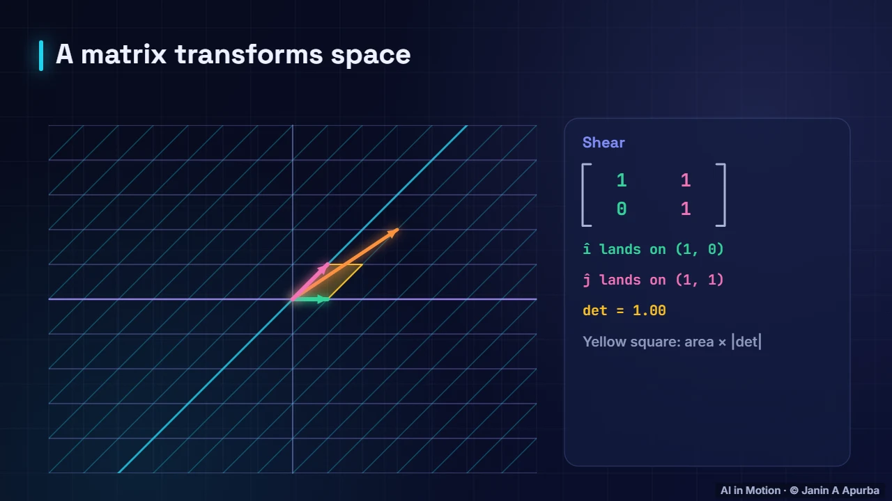
Columns are destinations. Here is the column view in pictures. The first column says where the basis vector i hat lands, and the second says where j hat lands. This shear matrix keeps i hat in place but tips j hat over to one, one, and the whole grid follows along.
Linearity. Matrices perform linear maps. Grid lines stay straight, parallel and evenly spaced, and the origin stays fixed. In algebra, the transform of a sum is the sum of the transforms. That is why knowing where the basis vectors land tells you where every single vector lands.
Rotation. A rotation is also a matrix. Its columns are zero, one and minus one, zero, which sends i hat straight up and j hat to the left. Every vector turns by ninety degrees. Rotations keep lengths and angles intact, so the yellow square keeps its area.
Scaling. A diagonal matrix stretches or squashes along the axes. This one doubles every x coordinate and halves every y coordinate. Feature scaling in machine learning, where each input column is multiplied by its own factor, is exactly a diagonal matrix like this one.
Pause and think. Quick check. Where does the stretch and squash matrix, two, zero, zero, one half, send the vector one, four? Think of it row by row. The answer is two, two: the x component is doubled to two, and the y component is halved to two.
Reflection. A reflection flips space like a mirror. This matrix sends i hat to minus one, zero and leaves j hat alone, so everything is mirrored across the vertical axis. Lengths are preserved, but left and right are swapped. Keep an eye on the yellow square, because orientation is about to matter.
Determinant. The determinant tells you how much a matrix scales area. For a two by two matrix it is a times d minus b times c. A determinant of three triples every area. A negative determinant flips orientation, like a mirror. And a determinant of zero squashes space flat.
Pause and think. Pause and think. What is the determinant of the shear matrix we saw earlier, one, one, zero, one? It is one times one minus one times zero, which equals one. The shear slants the square into a parallelogram, but the area stays exactly the same.
Squashing space. Here is a matrix with determinant zero: one times one minus two times one half. Both basis vectors land on the same line, so the whole plane collapses onto that line. Different inputs end up at the same output, and there is no way to undo it.
Inverse. The inverse of a matrix undoes it, returning every vector to where it started. It exists only when the determinant is not zero, because you cannot unsquash a flattened space. Solving a system of linear equations is the same as applying an inverse, though in practice we use stable solvers.
Linear regression in matrix form. Inverses appear in a classic formula. The least squares weights of linear regression are X transpose X, inverted, times X transpose y. These are called the normal equations. With millions of rows we switch to gradient descent, but for modest data this single matrix formula gives the exact answer.
Regression as a projection. Geometrically, linear regression projects the vector of targets onto the space spanned by the feature columns. The fitted line is the closest point in that space, and the residuals, the gaps between the points and the line, are perpendicular to it. Matrix algebra and geometry tell the same story.
Rank. Rank counts how many independent directions a matrix can produce. A full rank two by two matrix covers the whole plane. The singular matrix we just saw has rank one. Low rank matrices are cheap to store, an idea that fine tuning methods like LoRA exploit.
Low rank in practice. LoRA is a beautiful use of rank. Instead of updating a huge weight matrix during fine tuning, it learns the change as the product of two thin matrices of small rank. Far fewer numbers need to be trained and stored, yet the adapted model performs well.
Matrix multiplication. Multiplying two matrices, A times B, gives a new matrix C. Each entry of C is the dot product of a row of A with a column of B. Watch the cells fill one by one. The inner sizes must match: a two by three matrix times a three by two gives two by two.
Composition. Why multiply matrices at all? Because applying one transformation after another is itself a single matrix: the product. Here we rotate by ninety degrees and then stretch. The combined effect equals the single matrix B times A. Note that order matters: rotate then stretch differs from stretch then rotate.
Pause and think. Pause and think. Is matrix multiplication commutative? In other words, is A times B always equal to B times A? The answer is no. Rotating and then stretching gives a different result from stretching and then rotating, and sometimes the shapes do not even allow the reverse product.
Layers are matrices. Now to neural networks. Each layer of a network takes a vector of activations and multiplies it by a weight matrix, adds a bias vector, and applies an activation function. The arrows between two layers are exactly the entries of one weight matrix.
A layer in one line. A whole dense layer fits in one line: h equals sigma of W x plus b. W has one row per output neuron. The activation function sigma is essential. Without it, stacking many layers would just multiply matrices together, collapsing into one single linear layer.
Pause and think. Here is a deeper question. Why would a ten layer network without any activation functions be no more powerful than a single layer? Because the product of all ten weight matrices is itself just one matrix. Composing linear maps always gives another linear map.
Parameter counts. The size of a weight matrix is the number of inputs times the number of outputs, plus one bias per output. A small digit classifier layer has about one hundred thousand parameters. A single projection inside a seven billion parameter language model has around seventeen to forty five million.
Batches. Matrices also let us process many examples at once. Stack a batch of input vectors as the rows of a matrix, and a single matrix multiplication handles the whole batch. That is why GPUs, which excel at huge matrix products, made deep learning practical.
In code. In code, the at operator multiplies matrices. The two by three matrix times the three by two matrix gives the same answer we animated. Then a layer’s weights and a batch of sixty four inputs are processed with one matrix multiplication followed by a ReLU.
Special matrices. Some matrices are worth recognising on sight. The identity changes nothing. Diagonal matrices scale each axis. Orthogonal matrices rotate without changing lengths. Symmetric matrices, like covariance matrices, have real eigenvalues. And low rank matrices squeeze everything into a few directions.
Transpose. The transpose flips a matrix over its diagonal, turning rows into columns. It shows up constantly: a dot product is a transpose times a vector, covariance matrices are X transpose X, and backpropagation sends error signals backwards through a layer using the transposed weight matrix.
Matrices in backpropagation. During training, gradients flow backwards through the same computational graph. For a matrix layer, the gradient with respect to the input is the transposed weight matrix times the incoming gradient. So the forward pass and the backward pass are both matrix products.
Attention is a matrix. Attention weights themselves form a matrix: one row for each word that is looking, one column for each word it looks at. Multiplying this matrix by the matrix of value vectors mixes information between positions. A transformer layer is essentially a carefully arranged sequence of matrix products.
Transformations everywhere. Matrices appear throughout AI. An embedding table is a matrix with one row per token. Attention creates queries, keys and values with three projection matrices. Transformer MLP blocks are two big matrices. PCA is a rotation, and computer vision is full of geometric transformations.
Pause and think. One more question. A matrix maps three dimensional inputs to two dimensional outputs. Can it have an inverse? No. It is not square, and it necessarily loses information, because many different inputs share each output. Only square matrices with non zero determinant can be inverted.
Common pitfalls. Watch out for common pitfalls. Shape errors are the most frequent bug in deep learning code, so always check inner sizes. Remember that order matters. In NumPy the star operator multiplies element by element, while the at operator is the matrix product. And prefer a solver over computing an inverse.
Recap. To recap. A matrix is a linear transformation of space, and its columns show where the basis vectors land. The determinant measures area scaling, and zero means space is squashed and cannot be inverted. Multiplying matrices composes transformations, and every dense layer computes sigma of W x plus b.