Eigenvectors, SVD and PCA
Find the directions a matrix does not turn, break any matrix into rotate–stretch–rotate, and use it to compress data with principal component analysis.
📄 Illustrated notes · every chapter as a picture · printable
Quick quiz
5 questions to check your understanding.
Go deeper
University-level written lectures in The AI Lecture Hall:
Transcript
Introduction. This deep dive is about the hidden axes inside matrices. Eigenvectors reveal the directions a transformation does not turn. The singular value decomposition breaks any matrix into simple steps. And principal component analysis uses both to compress data. These ideas appear all over machine learning.
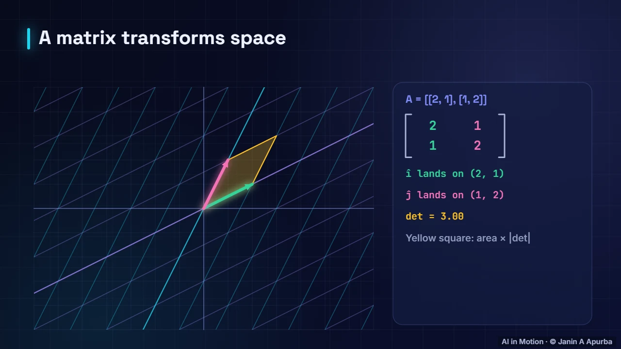
Most vectors turn. Watch this matrix transform the plane. Most vectors get knocked off their original line: the orange vector starts pointing right, and ends up pointing up and to the right. But are there special directions that do not turn at all, and only get stretched?
Eigenvectors. Yes. These are the eigenvectors. Along the diagonal direction one, one, every vector is simply stretched by three. Along the direction one, minus one, vectors keep their length, a stretch of exactly one. All the other arrows turn. The stretch factors, three and one, are called eigenvalues.
The eigen equation. In symbols, A times v equals lambda times v. Applying the whole matrix to an eigenvector gives the same result as multiplying it by a single number, lambda, the eigenvalue. A negative lambda flips the vector around, and a lambda of zero squashes that direction completely.
Finding them. How do we find them? Eigenvalues solve the equation determinant of A minus lambda times the identity equals zero. For our matrix that gives two minus lambda, squared, minus one equals zero, so lambda is three or one. Then each eigenvector comes from solving a small linear system.
Pause and think. Pause and think. A rotation by ninety degrees turns every single vector. How many real eigenvectors can it have? The answer is none. No direction stays on its own line, so there is no real solution. Its eigenvalues turn out to be complex numbers.
Symmetric matrices. Symmetric matrices, which equal their own transpose, are especially well behaved. The spectral theorem says they always have real eigenvalues and perpendicular eigenvectors. So they can be written as a rotation, a stretch along the axes, and the rotation back. Covariance matrices are symmetric, which matters for PCA.
Diagonalisation. This is called diagonalisation: A equals Q times lambda times Q transpose. In the eigenvector coordinate system, the matrix is just a stretch along each axis. One bonus is that powers become easy, since applying A ten times just raises each eigenvalue to the tenth power.
Eigenvectors in the wild. Eigenvectors appear in surprising places. This weather Markov chain settles into a long run distribution of about forty six percent sunny, twenty eight percent cloudy and twenty six percent rainy. That stationary distribution is an eigenvector of the transition matrix, with eigenvalue one. Google’s original PageRank used the same idea.
Pause and think. Pause and think. Some direction has eigenvalue one half. What happens to that component if we apply the matrix ten times? It gets multiplied by one half to the power ten, about one thousandth, so it almost vanishes. Eigenvalues above one make components grow, and those below one make them shrink.
Power iteration. That observation gives a simple algorithm called power iteration. Start with any vector, multiply by the matrix again and again, and rescale each time. The component with the largest eigenvalue grows fastest and soon dominates. PageRank used this idea to rank billions of web pages.
Eigenvalues as curvature. Eigenvalues also describe the shape of a loss surface. Near a minimum, the loss is approximately a bowl whose curvature along each direction is an eigenvalue of the Hessian matrix. Here one direction is eight times steeper than the other, which is exactly why gradient descent zig zags.
Condition number. The ratio of the largest to the smallest eigenvalue is the condition number. A large condition number means a long, narrow valley, where one learning rate is too big for one direction and too small for another. Feature scaling, batch normalisation and adaptive optimisers all help by taming it.
Beyond square matrices. Eigenvectors only work for square matrices, and not even all of those. The singular value decomposition works for every matrix of any shape. It says any matrix can be written as a rotation, then a stretch along the axes, then another rotation. The stretch factors are called singular values.
Rotate, stretch, rotate. Watch the unit circle. First V transpose rotates it, lining up two special input directions with the axes. Then sigma stretches along the axes, by about two point three eight and one point two six. Finally U rotates the result. The circle becomes an ellipse, exactly as the original matrix would do.
Rank-one pieces. Another way to read the SVD: any matrix is a sum of simple rank one pieces, each weighted by a singular value, sorted from most to least important. Keeping only the top k pieces gives the best possible rank k approximation. This is the mathematical heart of compression.
Singular values decay. In real data, singular values usually fall off quickly. For a typical photograph, the first few carry most of the structure and the rest describe fine detail and noise. That is why keeping a small number of components can reproduce an image, or a dataset, surprisingly well.
Pause and think. Pause and think. A grayscale image is a thousand by a thousand matrix. Roughly how many numbers are needed to store its rank twenty approximation? Each piece needs a column of a thousand, a row of a thousand and one singular value, so about forty thousand numbers, instead of one million.
PCA. Now to principal component analysis. PCA finds the perpendicular directions along which the data varies the most, called principal components, and projects the data onto the top few. You might compress a hundred correlated features into ten components while keeping most of the variance.
PCA in action. Here PCA searches for the direction of maximum spread. The first principal component points along the long axis of the cloud. Projecting onto it keeps most of the information in one number per point. The second component, perpendicular to the first, captures what remains.
The PCA recipe. Here is the PCA recipe. Centre the data by subtracting each feature’s mean. Compute the covariance matrix. Find its eigenvectors, or equivalently take the SVD of the data. Sort the directions by eigenvalue, which is the variance they explain, and project onto the top ones.
Why eigenvectors?. Why do eigenvectors appear? The variance of the data projected onto a unit direction w is w transpose C w. Maximising that is exactly solved by the top eigenvector of the covariance matrix, and its eigenvalue is the variance it captures. PCA is an eigenvalue problem.
Explained variance. A scree plot shows how much variance each component explains. In this example the first component explains sixty two percent, the second twenty one, and the third nine. The first three together keep ninety two percent of the variance, so three numbers per example might be enough.
In code. In code, scikit learn makes PCA a two liner. Ask for enough components to keep ninety five percent of the variance, fit, and transform. You can inspect how much variance each component explains. Under the hood it is an SVD of the centred data, which you can call directly with NumPy.
Eigenvectors in NumPy. In NumPy, the eigh function handles symmetric matrices quickly and stably. For our matrix it returns eigenvalues one and three, with the unit eigenvectors as the columns of a matrix. Multiplying A by the second eigenvector gives exactly three times that vector, confirming the definition.
PCA: strengths and limits. PCA is great for compressing correlated features, visualising high dimensional data and removing noise. But it only finds linear structure, it is sensitive to feature scale, so standardise first, and components can be hard to interpret. For curved structure, methods like t SNE or UMAP help with visualisation.
Pause and think. Pause and think. You forget to standardise, and one feature is income in dollars, with enormous variance, while the others are small ratios. What will the first principal component be? Almost exactly the income axis. PCA chases raw variance, so the biggest scale wins. Always standardise first.
Beyond PCA. The same mathematics powers many applications. Recommender systems factor a user by item matrix into a low rank product. LoRA learns low rank updates. Latent semantic analysis takes the SVD of a term document matrix. Spectral clustering uses eigenvectors of a graph, and eigenvalues explain exploding signals in deep networks.
Low rank in fine-tuning. Low rank structure also explains why parameter efficient fine tuning works. The LoRA authors found that the change a large pre-trained model needs to adapt to a new task has a low intrinsic rank. So instead of a full update, they learn two thin matrices, and very small ranks, such as four or eight, often work well.
Summary table. To compare the two. Eigen decomposition works for square, diagonalisable matrices, and its eigenvalues can be negative or even complex. The SVD works for any matrix, and its singular values are never negative. For symmetric positive matrices like covariance matrices, the two coincide.
Recap. To recap. Eigenvectors are directions a matrix only stretches, and eigenvalues are the stretch factors. Symmetric matrices have perpendicular eigenvectors. The SVD writes every matrix as rotate, stretch, rotate, and its top pieces give the best low rank approximation. PCA is simply eigenvectors of the covariance matrix.