Word Embeddings: A Deep Dive
How words became vectors: one-hot and TF-IDF, the distributional hypothesis, word2vec skip-gram with negative sampling, analogies, GloVe and fastText, contextual embeddings from BERT, sentence embeddings for search, and bias.
📄 Illustrated notes · every chapter as a picture · printable
Quick quiz
5 questions to check your understanding.
Go deeper
University-level written lectures in The AI Lecture Hall:
Transcript
Introduction. Computers work with numbers, but language is made of words. How do we turn words into numbers that capture meaning, so that cat is close to kitten and far from carburettor? In this deep dive we trace the answer, from simple counts to word2vec and the contextual embeddings inside modern language models.
The representation problem. Every language model begins by turning words into numbers, and that choice shapes everything that follows. A representation can capture only which word it is, how often it appears, or something much richer: what the word means and how it relates to other words.
One-hot vectors. The simplest representation is one hot encoding: a vector as long as the whole vocabulary, all zeros except for a single one at the word’s position. With fifty thousand words, every word becomes a fifty thousand dimensional vector with just one non zero entry.
Pause and think. Pause and think. What is the cosine similarity between the one hot vectors for cat and kitten? And between cat and carburettor? Both are exactly zero, because one hot vectors are all perpendicular to each other. They carry no notion of similarity at all.
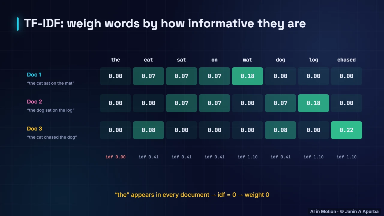
Counting words. For whole documents, a bag of words counts how often each word appears, throwing word order away. Common words like the dominate the counts, so TF IDF reweights them. Words that appear in every document get an inverse document frequency of zero, while rare, distinctive words like mat, log and chased get the highest weights.
TF-IDF. TF IDF multiplies a word’s frequency in a document by the log of the total number of documents divided by the number containing the word. A word that is frequent here but rare elsewhere is distinctive, so it scores high. These vectors are still sparse, and they still ignore meaning.
Compute an IDF. Let us compute an inverse document frequency. A word appears in ten of one thousand documents. The natural log of one thousand over ten, that is of one hundred, is about four point six. A word that appears in all one thousand documents gets the log of one, which is zero.
The key idea. The breakthrough idea is older than computers: words that occur in similar contexts tend to have similar meanings, an idea associated with linguists Zellig Harris and J R Firth in the nineteen fifties. Coffee, tea and cocoa all fit in I drank a cup of blank, so they should end up with similar representations.
Dense embeddings. A word embedding is a short, dense vector of real numbers, typically one to three hundred numbers, learned so that words used in similar contexts get similar vectors. Instead of fifty thousand mostly zero entries, each word gets a compact description in which every dimension carries some information.
Training pairs. Word2vec learns embeddings from raw text. Slide a window across the text. For each centre word, every neighbour within two positions becomes a training pair: quick predicts the, brown and fox. Millions of such pairs teach the network which words appear in similar contexts.
word2vec. Word2vec, published in 2013, is a shallow network with two flavours. Skip gram predicts the context words from the centre word, and continuous bag of words predicts the centre word from its context. After training, the network’s input weights are the word embeddings. It could learn from billions of words in hours.
Negative sampling. Computing a softmax over the whole vocabulary for every pair would be slow, so word2vec uses negative sampling. For each real pair it pushes the dot product of the two vectors up, and for a handful of randomly sampled negative words it pushes their dot products down. Five or so negatives per pair is enough.
A space of meaning. After training, each word is a point in space. We draw two dimensions here, but real embeddings have hundreds. Words used in similar ways end up close together: fruit near fruit, animals near animals, royalty near royalty. Nobody labelled these groups; they emerged from context alone.
Analogies. Even directions carry meaning. The step from man to woman points roughly the same way as the step from king to queen. So king minus man plus woman lands close to queen. This famous example from word2vec showed that relationships, not just words, are captured as geometry.
Measuring similarity. Similarity between embeddings is measured with the dot product, usually normalised into cosine similarity. It is large when two vectors point in similar directions, zero when they are unrelated and negative when they point in opposite directions. Here the two vectors are forty five degrees apart.
Pause and think. Pause and think. When you compute king minus man plus woman and search for the nearest word, why is king itself usually excluded? Because the resulting vector often stays closest to one of its inputs. Standard analogy tests exclude the three input words, and then queen comes out on top.
GloVe. GloVe, from Stanford in 2014, takes a different route to similar results. It first counts how often every pair of words co occurs across the whole corpus, then learns vectors whose dot products match the logarithm of those counts. It combines the global statistics of counting with the efficiency of learned vectors.
fastText. FastText, from Facebook in 2016, represents each word as the sum of vectors for its character pieces. Unhappiness shares pieces with unhappy and happiness, so even rare, misspelled or completely new words get sensible vectors. This helps greatly in languages with rich word forms.
Static embeddings compared. In summary, word2vec learns by predicting nearby words and is fast with strong analogies. GloVe fits global co occurrence statistics. FastText builds words from character pieces, handling rare and unseen words. All three give each word a single, fixed vector.
The limitation. That is also their main limitation. A static embedding gives bank exactly the same vector in river bank and in bank account, so its different senses are blended together. The vector sits somewhere between money and rivers, and the model must work out the meaning some other way.
Pause and think. Pause and think. In she sat on the bank and watched the river, what must a model use to choose the right sense of bank? The surrounding words, sat, watched and river. We need a representation that changes with context, and that is exactly what contextual embeddings provide.
Contextual embeddings. BERT, from 2018, produces contextual embeddings. It is trained by hiding words and predicting them from both sides: the chef cooked a something dinner for us. Every word’s vector is computed from the whole sentence, so bank gets different vectors next to river and next to money.
How context flows in. The mechanism is attention. Each word looks at every other word and pulls in information from the most relevant ones. Here the word it attends mostly to animal. After many layers of this mixing, each vector describes the word as it is used in this particular sentence.
Evaluating embeddings. How do we judge an embedding? Intrinsic tests check whether its similarities agree with human ratings, or how many analogies it solves. Extrinsic tests measure what really matters: performance on a downstream task such as classification or search. The two do not always agree, so test on your own task.
Sentence embeddings. Often we need a vector for a whole sentence or passage. Models such as Sentence BERT, from 2019, are trained so that texts with similar meaning land close together, even when they share no words. These sentence embeddings are the backbone of semantic search and retrieval augmented generation.
Semantic search. Here is semantic search at work. Every help article is embedded as a vector. The query, I can’t sign in, shares no words with reset your password or forgot login details, but its embedding lands right next to them, so they are returned as the top results.
Seeing embeddings. Embeddings have hundreds of dimensions, so to look at them we project them down. PCA finds the directions of greatest variance, as shown here, while methods like t SNE and UMAP preserve local neighbourhoods. Such plots are useful for exploring, but be careful: distances in two dimensions can mislead.
Bias. Embeddings learn from human writing, and they absorb its stereotypes too. A 2016 study found analogies such as man is to computer programmer as woman is to homemaker. Debiasing methods help only partly, so systems built on embeddings must be audited for unfair behaviour.
Pause and think. Pause and think. A résumé filter ranks applicants by embedding similarity to past successful hires. What could go wrong? It can reproduce historical bias: if past hires were skewed towards one group, words associated with that group score higher. Outcomes must be audited across groups.
In code. Training word2vec yourself takes a few lines with gensim. Provide tokenised sentences, ideally millions of them, choose skip gram with a hundred dimensions, a window of five and five negative samples, then look up vectors, nearest neighbours and analogies. Pre trained embeddings are also freely available.
Where embeddings are used. Embeddings are everywhere. Search engines find documents by meaning rather than exact keywords. Recommender systems embed products and songs as vectors too. Clustering groups similar texts to discover topics, and embeddings serve as input features for classifiers and as the first layer of every language model.
Recap. To recap. One hot and TF IDF vectors are sparse and carry no notion of meaning. The distributional hypothesis led to dense embeddings like word2vec, GloVe and fastText, where analogies become directions. Contextual embeddings from BERT change with the sentence, and sentence embeddings power semantic search, but must be audited for bias.