Reinforcement Learning Foundations: Agents, MDPs and Returns
How an agent learns from rewards: the agent–environment loop, Markov decision processes, discounted returns, policies and value functions — the vocabulary behind every RL algorithm.
📄 Illustrated notes · every chapter as a picture · printable
Quick quiz
5 questions to check your understanding.
Go deeper
University-level written lectures in The AI Lecture Hall:
Transcript
Introduction. Welcome to the first deep dive on reinforcement learning, the branch of AI where an agent learns by trial and error, guided only by rewards. It taught computers to play Atari from pixels, beat world champions at Go, and it shapes how chatbots are aligned with human preferences.
A different kind of learning. Supervised learning is like studying with an answer key: every example comes with the correct label. Reinforcement learning is different. Nobody tells the agent the right action. It only receives rewards, those rewards may arrive long after the decisions that earned them, and every action changes what the agent sees next.
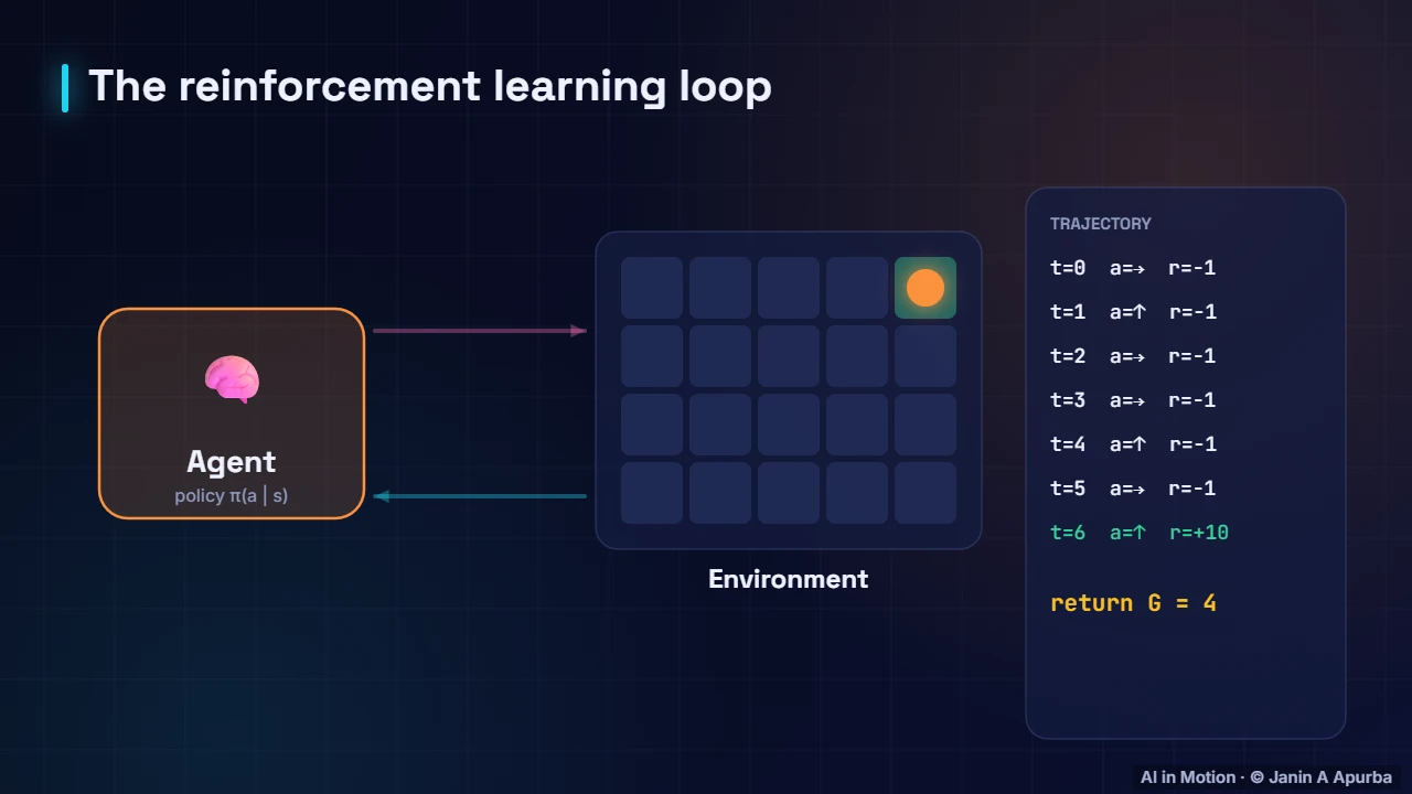
The agent–environment loop. Everything in reinforcement learning happens in a loop. The agent observes the state of the environment and chooses an action. The environment responds with a new state and a reward. Here each step costs minus one and reaching the star gives plus ten, so this trajectory earns a total of four.
The vocabulary. Let us fix the vocabulary. The state is what the agent observes, like a chess board. An action is a choice it can make, like a legal move. A reward is a number saying how good a step was. The policy is the agent’s strategy, and an episode is one complete run, like one game.
Milestones. The field has a remarkable history. In 1992 TD Gammon reached expert level at backgammon. In 2013 deep Q networks learned Atari games straight from pixels. AlphaGo beat Lee Sedol in 2016, AlphaZero mastered three board games from self play, and from 2022 reinforcement learning from human feedback shaped chat assistants.
A grid world. Here is the running example for this track: a small grid world. The agent starts in the bottom left corner. Reaching the green square gives plus one and ends the episode, falling into the red pit gives minus one, and every other step costs a little, minus point zero four, so dawdling is discouraged.
Stochastic environments. This world is also slippery. When the agent tries to move up, it succeeds eighty percent of the time, but ten percent of the time it slides to the left and ten percent to the right. Real environments are like this: robots slip, markets fluctuate and opponents surprise you.
Pause and think. Pause and think. The random agent has wandered for one hundred and sixty steps without reaching either exit. What is its total reward so far? Each step costs point zero four, so it has collected minus six point four. The small step penalty is what makes efficient paths worth learning.
The Markov property. Reinforcement learning usually assumes the Markov property: the future depends only on the current state and action, not on the history. A chess position has this property. A single frame of a video game does not, because you cannot tell which way the ball is moving, which is why game agents stack several frames.
Markov decision process. Formally, the environment is modelled as a Markov decision process, or MDP. It consists of a set of states, a set of actions, transition probabilities saying where each action might lead, a reward function, and a discount factor gamma. Almost every reinforcement learning algorithm is built on this model.
An MDP as a diagram. Here is a tiny MDP about a machine. Running it fast earns two points, running it slowly earns one. But running fast warms the machine half the time, and running fast while it is warm overheats it, which costs ten points and ends everything. The best policy must weigh reward now against risk later.
Return. The agent’s goal is not to maximise the next reward, but the return: the sum of all future rewards from now on. A chess player happily sacrifices a piece now to win the game later. Maximising the return is what makes reinforcement learning about long term planning.
Discounting. Usually future rewards are discounted. A reward t steps in the future is multiplied by gamma to the power t. With gamma of point nine, the plus ten reward four steps away is worth about six point five six today, and the whole return is about three point one two.
Choosing gamma. The discount factor sets how far ahead the agent looks. With gamma of one half, rewards more than a few steps away barely count. With point nine the effective horizon is about ten steps, and with point nine nine about a hundred. Discounting also keeps infinite sums finite.
Pause and think. Pause and think. Why would we choose gamma of point nine nine for chess rather than one half? Because chess is won or lost many moves later. With one half, the final reward would be practically invisible from the opening. A gamma close to one lets the agent value long term consequences.
Policy. The policy is the agent’s behaviour. A deterministic policy picks one action per state. A stochastic policy gives a probability for each action, which is useful for exploring and for games where being predictable is a weakness. It can be a lookup table or a large neural network.
State value. How good is it to be in a state? The state value function answers this: the expected return if you start in that state and follow the policy afterwards. In our grid world, states near the goal have high value, and states near the pit have low value.
Action value. The action value function, called Q, is even more useful. It is the expected return if you take a particular action first and then follow the policy. If you know Q, acting well is easy: in every state simply pick the action with the highest Q value. That is the idea behind Q learning.
Values in the grid world. Here are state values for our grid world, computed exactly, as we will learn in the next lecture. The cell next to the goal is worth about point nine three. Values fall as we move away, reaching almost zero at the start. Brighter green means a better place to be.
The Bellman equation. Values obey a beautiful recursive relationship called the Bellman equation. The value of a state equals the expected immediate reward, plus the discounted value of the next state. Today’s value is reward now plus the discounted value of tomorrow. Nearly every algorithm in this track exploits it.
Pause and think. Try the Bellman equation yourself. A state gives a reward of one, and always leads to a next state worth five. With gamma equal to point nine, what is the value of the first state? It is one plus point nine times five, which equals five and a half.
Optimality. The goal of reinforcement learning is an optimal policy: one that does at least as well as any other policy from every state. Every finite MDP has at least one. Its value functions are written V star and Q star, and finding them is the central problem of the field.
The families of algorithms. Algorithms fall into families. Model based methods know or learn how the world works and then plan. Value based methods learn Q values from experience and act greedily. Policy based methods adjust the policy directly. Actor critic methods combine a policy and a value function, and they dominate modern practice.
Explore or exploit?. Every learning agent faces a dilemma. Should it exploit what it already knows, collecting reward now, or explore something new that might be better? Exploit too much and you never discover the best option. Explore too much and you waste time. We devote a whole lecture to this trade off.
Credit assignment. Another fundamental challenge is credit assignment. When a reward finally arrives, which of the many earlier decisions deserve the credit or the blame? A chess game lost on move sixty may have been lost by a blunder on move twelve. Value functions and discounting are our main tools for sorting this out.
Where RL is used. Reinforcement learning is used well beyond games. Robots learn to walk and grasp, often in simulation first. Recommender systems optimise long term engagement. It has been applied to data centre cooling, chip design and traffic control. And it is a key ingredient in aligning large language models.
The loop in code. In code, the loop looks the same in almost every library. Gymnasium is the standard toolkit. Create an environment, reset it to get the first state, then repeatedly choose an action and step the environment, receiving the next state and reward, until the episode ends. Here the policy is random.
Random versus trained. This is CartPole, a classic benchmark: push the cart left or right to keep the pole upright, earning plus one for every step it stays up. A random policy, like the one in our code, lets the pole fall after about twenty three steps on average. By the end of this track you will know how to do far better.
Common pitfalls. Framing a problem well is half the battle. Agents are famous for reward hacking, finding loopholes that score points without doing what you meant. Sparse rewards give almost no signal. States that hide crucial information break the Markov assumption. And reinforcement learning is hungry, often needing millions of interactions.
Pause and think. A final question. You reward a cleaning robot plus one for every piece of dirt it picks up. What could go wrong? It might learn to tip out the dirt and pick it up again, forever. Reward the outcome you actually want, a clean room, rather than a proxy that can be gamed.
Recap. To recap. The agent and environment interact in a loop of states, actions and rewards, formalised as a Markov decision process. The goal is the discounted return, not the next reward. Value functions measure how good states and actions are, and the Bellman equation links the value now to the value next.