Packaging and Serving Models
From a model file to a reliable service: batch vs online inference, a FastAPI endpoint, Docker images, Kubernetes and autoscaling, latency percentiles and queueing, GPU batching, optimisation and edge deployment.
📄 Illustrated notes · every chapter as a picture · printable
Quick quiz
5 questions to check your understanding.
Go deeper
University-level written lectures in The AI Lecture Hall:
Transcript
Introduction. A trained model is just a file until something uses it. Serving is the engineering that turns that file into predictions for real users, quickly, reliably and affordably. In this deep dive we package a model, put it behind an API, containerise it and scale it.
The model artefact. The model artefact must contain everything needed to make a prediction: the learned weights, the preprocessing steps, the expected feature order, the label mapping and metadata such as library versions. A classic bug is saving the model but not the scaler that prepared its inputs.
Batch vs online. There are two basic ways to serve. Batch inference scores many records on a schedule, perhaps every night, and writes results to a table. It is simple and cheap. Online inference answers each request in real time through an API, which demands low latency and high availability.
Serving patterns. Choose the pattern by how fresh the prediction must be. Batch suits nightly scores. Online APIs suit decisions during a user action, like a fraud check while paying. Streaming handles continuous event flows, such as sensor data. On device inference gives instant, offline predictions, like keyboard suggestions.
Pause and think. Pause and think. The marketing team wants a churn risk score for every customer, refreshed daily, to plan emails. Which serving pattern fits? Batch inference. Score everyone overnight and store the results in a table. A real time API would add cost and complexity with no benefit.
An API with FastAPI. Here is an online prediction service in fifteen lines of Python with FastAPI. The model is loaded once, when the server starts. A schema validates every incoming request, rejecting malformed input. The versioned endpoint returns the probability together with the model version, which helps debugging later.
Pause and think. Pause and think. Why load the model at start up rather than inside the prediction function? Loading from disk can take seconds and a lot of memory. Doing it for every request would make every prediction painfully slow. Load once, then reuse the model for thousands of requests.
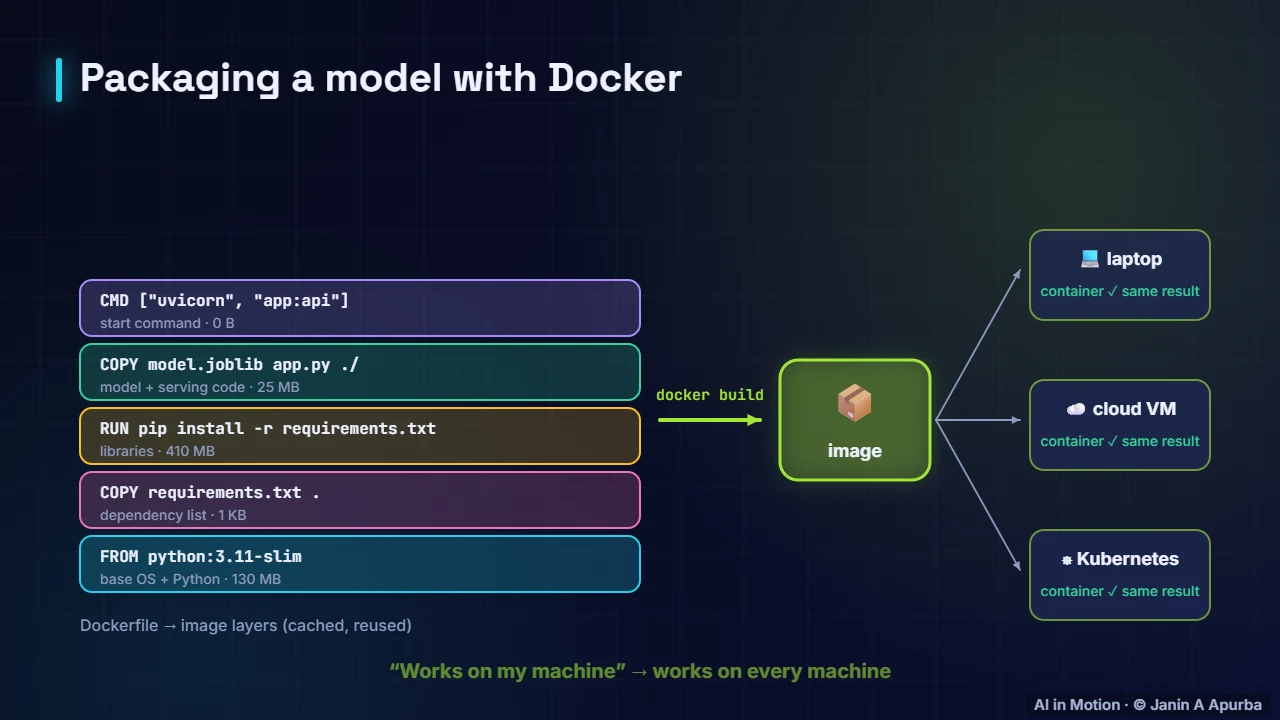
Containers. Next, package the service in a container. A Dockerfile builds an image layer by layer: a base image with Python, the dependency list, the installed libraries, the model and code, and the start command. The same image then runs identically on a laptop, a cloud virtual machine or a Kubernetes cluster.
The Dockerfile. The Dockerfile is short. Start from a small official Python image. Copy the requirements and install them first, so that this slow layer is cached and reused. Copy the model and code last, because they change most often. Finally, expose the port and start the web server.
Layer caching. Order matters because Docker caches layers. If a layer and everything before it are unchanged, Docker reuses it. By installing libraries before copying the application code, a one line code change rebuilds in seconds instead of reinstalling every library.
Orchestration. At scale, containers are run by an orchestrator, most often Kubernetes. You declare what you want, such as three replicas of version seven, and Kubernetes keeps it that way: restarting crashed containers, spreading them across machines, rolling out new versions gradually and scaling up or down with demand.
The request path. A request travels from the client to a load balancer, which spreads traffic across several identical replicas and skips unhealthy ones. The replicas report metrics such as CPU use and request rate, and an autoscaler adds replicas when load rises and removes them when it falls.
Autoscaling under real traffic. Here is a simulated day of traffic. As demand rises in the morning, the autoscaler adds replicas and latency stays low. Around midday a sudden burst arrives faster than new replicas can start, and the ninety fifth percentile latency jumps above the two hundred millisecond objective before capacity catches up.
Autoscaling config. Autoscaling is configured declaratively. This Kubernetes horizontal pod autoscaler targets the churn API deployment, keeps at least two replicas for availability and at most ten to cap cost, and adds replicas whenever average CPU use rises above sixty percent, leaving headroom for bursts.
Cold starts. Scaling is not instant. A new replica must start its container, load the model into memory, possibly onto a GPU, and warm up before serving. For large models this cold start can take minutes, which is why services keep a minimum of warm replicas and scale on early signals such as rising queue length.
Latency percentiles. Latency is measured with percentiles, not averages. The fiftieth percentile is the typical request. The ninety fifth and ninety ninth percentiles show the slow tail. A median of forty milliseconds can hide a ninety ninth percentile of nearly a second, which one user in a hundred experiences.
Pause and think. Pause and think. A page makes twenty independent model calls, and each has a one percent chance of being slow. How many page loads include at least one slow call? One minus point nine nine to the twentieth power, about eighteen percent. Tail latency compounds when requests fan out.
Queueing. Why does latency spike? Queueing theory gives a simple rule: in a basic queue, waiting time grows like one over one minus the utilisation. At half capacity, waits double. At ninety percent, they are ten times longer, and at ninety five percent, twenty times. So services are usually run well below full capacity.
Pause and think. Pause and think. Your service runs at eighty percent utilisation. Using the one over one minus rho rule, how much longer are waits than at fifty percent? At eighty percent the factor is five, and at fifty percent it is two, so waits are about two and a half times longer, and they explode beyond this point.
Latency budgets. How fast must a model be? Classic usability research gives three limits. About a tenth of a second feels instant. About one second keeps the user’s flow of thought. Around ten seconds is the limit of attention, beyond which you must show progress, or stream results as chatbots do.
GPU serving. Deep learning models are often served on GPUs, which are efficient only with batches. Servers such as NVIDIA Triton use dynamic batching: they hold incoming requests for a few milliseconds, group them, and run them together. A small latency cost buys a large gain in throughput and cost per prediction.
Optimising the model. The model itself can be optimised for serving. Export it to an optimised runtime such as ONNX Runtime or TensorRT, quantise weights to eight bit integers, prune unnecessary connections, or distil it into a smaller student model. These steps can make serving several times cheaper for a small accuracy cost.
Quantisation. Quantisation is often the easiest win. Storing weights in eight bit integers instead of thirty two bit floats cuts memory by four and speeds up inference on hardware with integer support. Calibration on sample data keeps the accuracy loss small, so always measure before and after.
CPU or GPU?. Not every model needs a GPU. Gradient boosted trees and small networks answer in well under a millisecond on ordinary CPUs, which are cheaper and simpler to operate. GPUs and other accelerators pay off for large neural networks and high throughput workloads.
Edge deployment. Some models run on the device itself, converted to formats such as TensorFlow Lite, Core ML or ONNX Runtime Mobile. Edge inference removes the network round trip, works offline and keeps personal data on the device. The trade off is tight limits on memory, power and model size.
Caching. Sometimes the fastest prediction is the one you do not compute. If the same inputs recur, cache the results for a while. Recommendations for a user can be cached for a few minutes, and predictions for common cases can be precomputed in batch and simply looked up.
Load testing. Before launch, load test. Tools such as Locust or k6 simulate realistic and peak traffic against the service, measuring throughput, tail latency and where it breaks. Test at two or three times the expected peak, and watch the ninety ninth percentile latency, error rates and memory, not just averages.
Serving many models. Real systems often serve many models: one per country, per customer segment, or two versions side by side during a migration. Multi model servers host many models, load them on demand and route each request by name and version, sharing hardware efficiently.
API design. Design the API carefully. Version the endpoints, so clients can migrate gradually. Validate inputs with strict schemas and clear error messages. Return metadata such as the model version and confidence. And set timeouts, with a sensible fallback answer when the model is slow or unavailable.
Reliability. Reliability comes from a few habits. Health check endpoints let the orchestrator know when a replica is ready or stuck. Graceful degradation falls back to simple rules if the model fails. Rate limiting protects against overload and abuse, and authentication and encrypted traffic keep the service secure.
Pause and think. Pause and think. The fraud model’s server goes down during a big sale. What should the payment system do? Fail gracefully: switch to a simple rule based fallback with conservative thresholds, log the event and alert the on call engineer. Blocking every payment, or approving everything blindly, would both be disasters.
Recap. To recap. Package the whole prediction pipeline. Choose batch, online, streaming or edge serving by how fresh predictions must be. A common stack is FastAPI, Docker and Kubernetes. Watch tail latency and keep utilisation well below capacity, and optimise with batching, quantisation, caching and the right hardware.