Monitoring, Drift and Retraining
Why models decay and how to catch it: what to monitor, data drift vs concept drift, the population stability index, delayed labels, alerting, incident response and retraining strategies.
📄 Illustrated notes · every chapter as a picture · printable
Quick quiz
5 questions to check your understanding.
Go deeper
University-level written lectures in The AI Lecture Hall:
Transcript
Introduction. A model is trained on a snapshot of the past, but it serves in a present that keeps changing. Customers change, markets change, sensors age and upstream systems get modified. In this deep dive we learn how to watch a model in production, detect when it drifts, and decide when to retrain.
Model decay. Model decay is the gradual, or sometimes sudden, loss of real world performance after deployment. The model itself does not change, but the world does, or an upstream pipeline does. A fraud model trained before a new payment method launches may simply not recognise the new patterns.
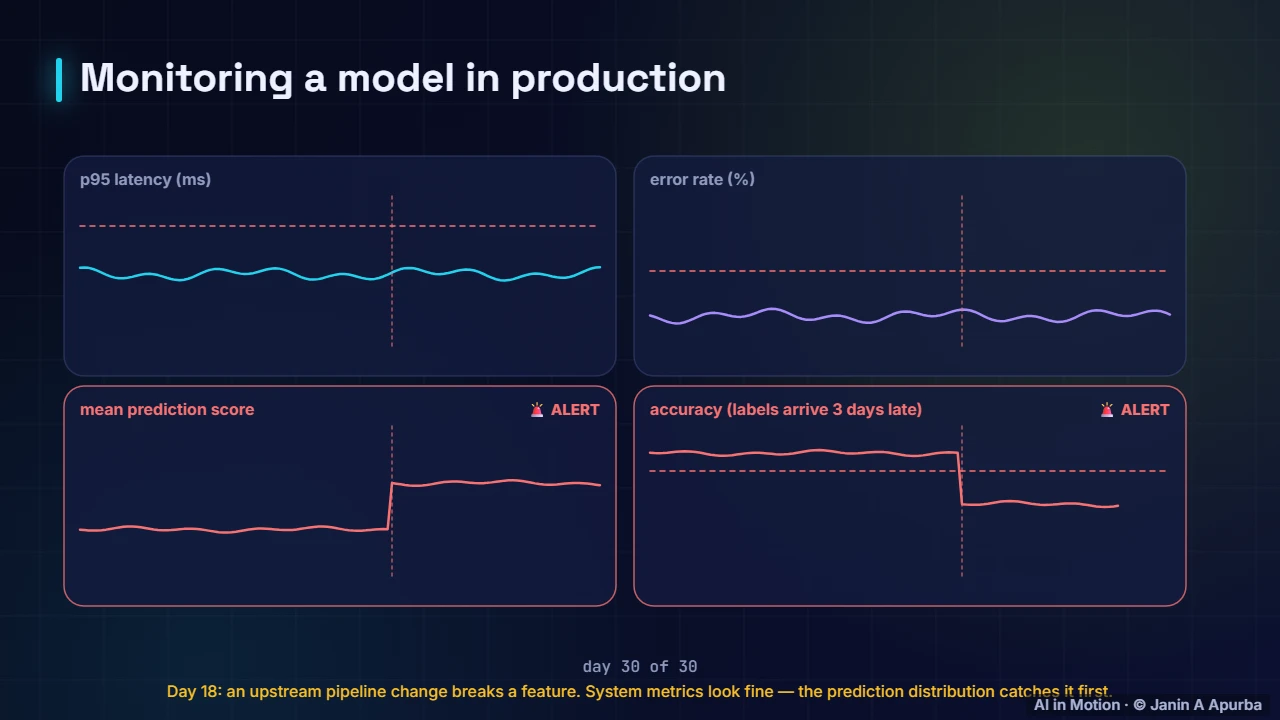
A monitoring dashboard. Here is a monitoring dashboard over thirty days. Latency and error rate stay perfectly healthy throughout. But on day eighteen an upstream pipeline change breaks a feature, and the mean prediction score jumps immediately. Accuracy, which can only be measured when labels arrive three days later, confirms the damage.
What to monitor. Monitor four layers. System metrics such as latency and errors. Data quality and feature distributions. The distribution of predictions. And outcomes: accuracy, business metrics and user feedback. The first three are available instantly. Outcomes often arrive days or weeks later, so the earlier layers are your early warning system.
Pause and think. Pause and think. In the dashboard, why did the prediction score panel sound the alarm before the accuracy panel? Because predictions are available instantly, while the true labels arrived three days later. Watching inputs and predictions gives early warning when outcomes are delayed.
Data drift. Data drift, also called covariate shift, is a change in the distribution of the inputs. Perhaps a bank’s app becomes popular with younger customers, so the age distribution shifts. The underlying relationship may be unchanged, but the model now sees more of the kinds of inputs it saw least during training.
Measuring drift. Here the live age distribution, in pink, slowly moves away from the training distribution, in blue. The population stability index, on the right, summarises the gap each week. It stays near zero at first, crosses the watch level of point one in week six, and passes the alert level of point two five in week eight.
The PSI formula. The population stability index splits the training data into ten equal bins, then compares the share of live data falling into each bin with the expected share. For each bin it multiplies the difference by the log of the ratio, and adds them up. It is closely related to a symmetric form of the KL divergence.
Pause and think. Pause and think. With the common rule of thumb, below point one is stable, point one to point two five is a moderate shift, and above that is significant. When would you act in our example? Start watching closely around week six, and investigate and probably retrain once the alert fires in week eight.
Other drift tests. Other measures are also common. The Kolmogorov Smirnov test compares continuous distributions, chi squared tests compare categories, and the Jensen Shannon distance is a bounded, symmetric divergence. Be careful with huge samples: statistical tests will flag tiny, harmless shifts, so look at effect sizes, not only p values.
Concept drift. Concept drift is more dangerous: the relationship between inputs and outcome changes, so the same inputs now mean something different. After an economic shock or a policy change, a customer profile that used to be low risk may now default more often. Input distributions can look perfectly normal while the model is wrong.
Data vs concept drift. In short, data drift changes what inputs look like. It is visible immediately, and the model may still be correct. Concept drift changes what inputs mean. It is invisible in the inputs, so detecting it needs outcome labels, or good proxies for them. Monitoring must cover both.
Pause and think. Pause and think. Fraudsters change their tactics after your model starts blocking their old pattern. Which kind of drift is this? Concept drift, and adversarial concept drift at that: transactions that look normal now carry a different risk. Expect it, watch outcomes closely and retrain frequently.
Label shift. A third kind is label shift: the frequency of outcomes changes, perhaps fraud becomes twice as common, while each class still looks the same. Rankings may remain good, but predicted probabilities and decision thresholds become miscalibrated, so recalibration is often enough.
Calibration. Also monitor calibration: whether predicted probabilities still match reality. Of all the cases scored at seventy percent risk, about seventy percent should turn out positive. After label shift, rankings may stay good while probabilities become badly wrong, which matters whenever decisions use thresholds or expected costs.
Pause and think. Pause and think. Every December your drift alerts fire for a retail model, then quietly stop in January. What is happening? Seasonality, not a broken model. Compare with the same period last year, or a seasonally adjusted baseline, and consider giving the model seasonal features.
Delayed labels. Outcomes are often delayed. Whether a loan defaults may take months, and some outcomes are never observed at all. In the meantime, use proxies such as complaints, overrides by staff or quick user feedback, and label a small random sample by hand each week to get an unbiased estimate of accuracy.
Alerting. Alerts turn monitoring into action. Alert on symptoms that matter, with thresholds tuned to avoid noise, and route each alert to a named owner with a runbook describing what to check. Too many false alarms cause alert fatigue, and then the one real alert gets ignored.
Service level objectives. Service level objectives make expectations explicit: for example, ninety fifth percentile latency under two hundred milliseconds, ninety nine point nine percent availability, and weekly sampled accuracy of at least point nine. An error budget says how much violation is tolerable before work must stop to fix reliability.
Incident response. When an alert fires, triage it: is it real, and how severe? Mitigate first, by rolling back or falling back to a simpler model. Then find the root cause: a data problem, a code change, or a genuine change in the world. Finish with a blameless post mortem that adds tests and better alerts.
Rollback as mitigation. Rollback is the fastest mitigation. Here a new version’s error rate climbs past its threshold during a canary release, and traffic automatically returns to the previous version. Keeping the last good model ready to serve turns a potential outage into a minor blip.
Retraining strategies. How often should you retrain? Scheduled retraining, such as weekly, is simple and predictable. Triggered retraining responds to drift or performance alerts. Online learning updates the model continuously as data arrives. The right choice depends on how fast the world changes and how costly and risky retraining is.
Retraining in action. This illustration shows the effect. A model that is never retrained slowly loses accuracy week after week. A model retrained every three weeks produces a sawtooth: accuracy slips between retrains, then recovers each time fresh data is incorporated.
Pause and think. Pause and think. Why not simply retrain every day, just to be safe? Retraining costs compute, needs fresh validated labels, and every new model is a chance to introduce a bug or regression. Retrain as often as the drift requires, and always through the same quality gates.
Backtesting. How do you choose a retraining schedule? Backtest it. Replay history: at each past date, train only on data available at that time, then measure performance on what came next. Comparing weekly, monthly and drift triggered retraining this way turns a guess into evidence.
System health still matters. Do not forget the system layer. Here traffic, capacity and latency are tracked through a day. A burst around midday pushes latency above the objective before the autoscaler catches up. Many model incidents turn out to be plain infrastructure problems, so system and model monitoring belong on the same dashboard.
Fairness over time. Monitor important segments separately: regions, devices, customer types and, where lawful and appropriate, demographic groups. An overall average can stay flat while performance collapses for one group, such as users of a new app version. Segment monitoring also supports fairness commitments.
A drift check. A drift check fits in a few lines. Build bin edges from the training data’s quantiles, compute the share of training and live data in each bin, guard against zeros, and sum the PSI terms. When the index crosses the alert threshold, notify the owner. Libraries such as Evidently package many such checks.
Logging for monitoring. All of this depends on logging. Record inputs, predictions, the model version and request metadata, sampled if volume is huge, and protect personal data. Later these logs are joined with outcomes to compute accuracy. Without them, drift and accuracy simply cannot be measured after the fact.
Best practices. To summarise the practice. Monitor all four layers. Compare live data with the training baseline, not only with last week, to catch slow drift. Alert on what matters, with owners and runbooks. Keep rollback and fallbacks ready. And retrain through the same gates as any other release.
Recap. To recap. Models decay because the world and the data pipelines change. Monitor systems, data, predictions and outcomes. Data drift changes the inputs, while concept drift changes what they mean. PSI summarises distribution shift, and when things go wrong, mitigate first, then fix the root cause and retrain.