Diffusion Models: The Complete Deep Dive
How image generators really work: the forward noising process and its schedule, the noise-prediction objective, U-Net denoisers, DDPM vs DDIM sampling, latent diffusion with a VAE, text conditioning with CLIP and cross-attention, classifier-free guidance, ControlNet and fast samplers.
📄 Illustrated notes · every chapter as a picture · printable
Quick quiz
5 questions to check your understanding.
Go deeper
University-level written lectures in The AI Lecture Hall:
Transcript
Introduction. Type a sentence and receive a detailed picture in seconds. Behind most modern image, video and audio generators sits one idea: diffusion. In this deep dive we go through it carefully, from the mathematics of adding noise to the tricks that make text to image systems like Stable Diffusion work.
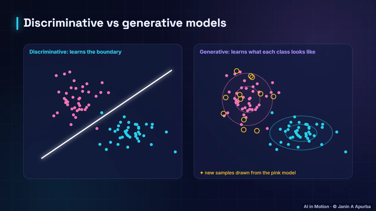
Generative modelling. First, recall what a generative model is. A discriminative model only learns the boundary between classes. A generative model learns what the data itself looks like, a whole probability distribution, so it can draw brand new samples from it. Diffusion models are an especially powerful way to learn such a distribution.
The big idea. The big idea is surprisingly simple. Take training images and slowly destroy them by adding a little noise at a time, until nothing but static remains. Then train a neural network to undo one small step of noising. To generate, start from pure noise and apply the network again and again.
A short history. The idea was proposed in 2015, but it took until 2020, with denoising diffusion probabilistic models, known as DDPM, to produce high quality images. In 2021 guided diffusion beat GANs on ImageNet. 2022 brought Stable Diffusion, DALL E two and Imagen to the public, and by 2024 text to video models had arrived.
Gaussian noise. The noise used is Gaussian: each pixel gets a random nudge drawn from a bell shaped normal distribution with mean zero. Gaussian noise has convenient mathematical properties. Adding many small Gaussian nudges is itself Gaussian, which is what makes the whole process tractable.
One noising step. One step of the forward process shrinks the previous image slightly and adds a small amount of Gaussian noise. The amount is set by beta t, which grows from about one ten thousandth to two hundredths across a thousand steps. After enough steps, all the original structure is gone.
The noise schedule. Here is that schedule. The green curve shows how much of the original image survives at each step. At step two hundred and fifty, about seventy two percent of the signal remains. At step five hundred, about twenty eight percent. By the final step, almost nothing is left: pure noise.
Jump to any step. Conveniently, we never need to add noise step by step. There is a closed form: the noisy image at step t is a mix of the clean image, scaled by the square root of alpha bar t, and fresh Gaussian noise. Alpha bar is simply the product of the one minus beta terms up to that step.
Pause and think. Pause and think. At step five hundred the signal factor is about point two eight. What does the image look like? Mostly noise. The clean image contributes a weight of point two eight, while the noise contributes about point nine six. Only faint, large scale shapes survive.
Learning to reverse. The reverse process is learned. A single neural network looks at a noisy image, together with the step number, and predicts the noise that was added. Subtracting a scaled version of that predicted noise moves the image one step closer to a clean one. The same network is used at every step.
The training objective. The training loss is remarkably simple: the mean squared error between the noise we actually added and the noise the network predicts. There is no adversary and no tricky balancing act, which is why diffusion models train far more stably than GANs.
One training step. One training step goes like this. Pick a clean image and a random step between one and a thousand. Use the closed form to create the noisy version in one go. Ask the network to predict the noise, and take a gradient step on the squared error. Repeat millions of times across the dataset.
Pause and think. Pause and think. Why train the network to predict the noise, rather than the clean image directly? Given the noisy image, one determines the other, so they are equivalent. But the noise has the same simple scale at every step, which makes learning much better behaved.
Generating an image. Now generation. Start from pure random static. At each step, the network predicts which part of the picture is noise, and a little of it is removed. Slowly, large shapes appear, then details sharpen, until a clean image emerges that matches the prompt.
The denoiser: a U-Net. The denoising network is usually a U Net, originally designed for medical image segmentation. Its encoder shrinks the image to understand its content, and its decoder expands back to full resolution, with skip connections preserving fine detail. Newer systems increasingly use transformers instead.
Knowing the step. The network must know which step it is working on, because removing heavy noise and polishing fine details are very different jobs. The step number is converted into an embedding, much like a positional encoding, and injected throughout the network.
Faster sampling. Running a thousand network passes for every image is slow. DDIM, published in 2020, reinterpreted the reverse process so that steps can be skipped, producing good images in twenty to fifty steps. Many improved samplers followed, and distilled models need only a handful of steps, or even one.
Latent diffusion. Denoising full resolution pixels is expensive. Latent diffusion, the idea behind Stable Diffusion, first compresses images with a variational autoencoder, shrinking a five hundred and twelve pixel image into a sixty four by sixty four latent with four channels. Diffusion runs in that small space, and a decoder turns the result back into pixels.
Compression first. This is the autoencoder idea. The encoder squeezes an image into a small code, and the decoder rebuilds it. In latent diffusion the autoencoder is trained first, separately, so that its latent space keeps the perceptually important content while discarding imperceptible detail.
Compute the saving. Let us compute the saving. A five hundred and twelve pixel square colour image holds seven hundred and eighty six thousand, four hundred and thirty two numbers. Its latent holds sixteen thousand, three hundred and eighty four. That is forty eight times fewer numbers to denoise at every step.
Understanding the prompt. How does the model understand the prompt? A text encoder, often from CLIP, turns the words into embeddings. CLIP was trained on hundreds of millions of image caption pairs to place matching images and captions close together, so its text embeddings carry visual meaning.
Cross-attention. The prompt guides every denoising step through cross attention. Inside the network, image features act as queries and the prompt’s word embeddings act as keys and values. Each region of the image attends to the words that concern it, so the car becomes red and the house blue.
Different prompt, different image. A different prompt, starting from the same kind of noise, steers the denoising towards a completely different picture. And a different random starting noise with the same prompt gives a different variation, which is why generators can produce endless alternatives for one description.
Classifier-free guidance. To follow prompts closely, samplers use classifier free guidance. At each step, the model predicts the noise twice: once without the prompt, the grey arrow, and once with it, the blue arrow. Guidance moves further along the difference between them, strengthening the prompt’s influence.
The guidance formula. The guided estimate is the unconditional prediction plus w times the difference between the conditional and unconditional predictions. With w equal to one we get plain conditioning. Values around seven and a half are a common default, and the model learns both predictions by randomly dropping the prompt during training.
Pause and think. Pause and think. What happens with a very high guidance scale, say thirty? Images follow the prompt very literally, but become over saturated, harsh and less varied, with visible artefacts. Moderate values balance faithfulness to the prompt against natural looking images.
Negative prompts. A neat twist on guidance is the negative prompt. Instead of an empty prompt for the unconditional prediction, you describe what you do not want, such as blurry or low quality. Guidance then pushes the image away from those features as well as towards the positive prompt.
More control. Text is not the only control. Image to image starts from a partly noised photo instead of pure noise, preserving its layout. Inpainting regenerates only a masked region. ControlNet, from 2023, adds conditioning on edge maps, depth maps or human poses, so an image follows an exact structure.
Fewer steps. Research keeps cutting the number of steps. Distillation trains a student model to cover many denoising steps at once, and consistency models, from 2023, learn to map any noisy point straight to a clean image. Some systems now generate usable images in one to four steps, fast enough for real time use.
In code. With the Hugging Face diffusers library, generation takes a few lines. Load a Stable Diffusion pipeline, which bundles the text encoder, the U Net and the VAE. Call it with a prompt, a negative prompt, thirty denoising steps and a guidance scale of seven and a half, and save the image.
Beyond images. Diffusion now reaches far beyond still images. Video models denoise many frames together for consistent motion. Audio models generate music, speech and sound effects. Others create three dimensional shapes, and in science, diffusion models help design new proteins and molecules.
Responsible use. These tools raise serious questions. They can create convincing deepfakes of real people. There are unresolved debates about copyright, consent and imitating artists’ styles. Generated images can reproduce stereotypes. Watermarking and content credentials that record how an image was made are part of the response.
Recap. To recap. The forward process adds Gaussian noise on a schedule, and we can jump to any step in closed form. A network learns to predict the added noise with a simple squared error. Generation denoises from pure noise, latent diffusion works in a compressed space guided by text, and guidance adds control.