Backpropagation, Step by Step
The chain rule in action: compute values forward, then pass gradients backward through a tiny computational graph — with real numbers.
📄 Illustrated notes · every chapter as a picture · printable
Quick quiz
3 questions to check your understanding.
Go deeper
University-level written lectures in The AI Lecture Hall:
Transcript
Introduction. A network may have millions of weights. After a mistake, how do we know how to change each one? Backpropagation answers that efficiently, using the chain rule from calculus.
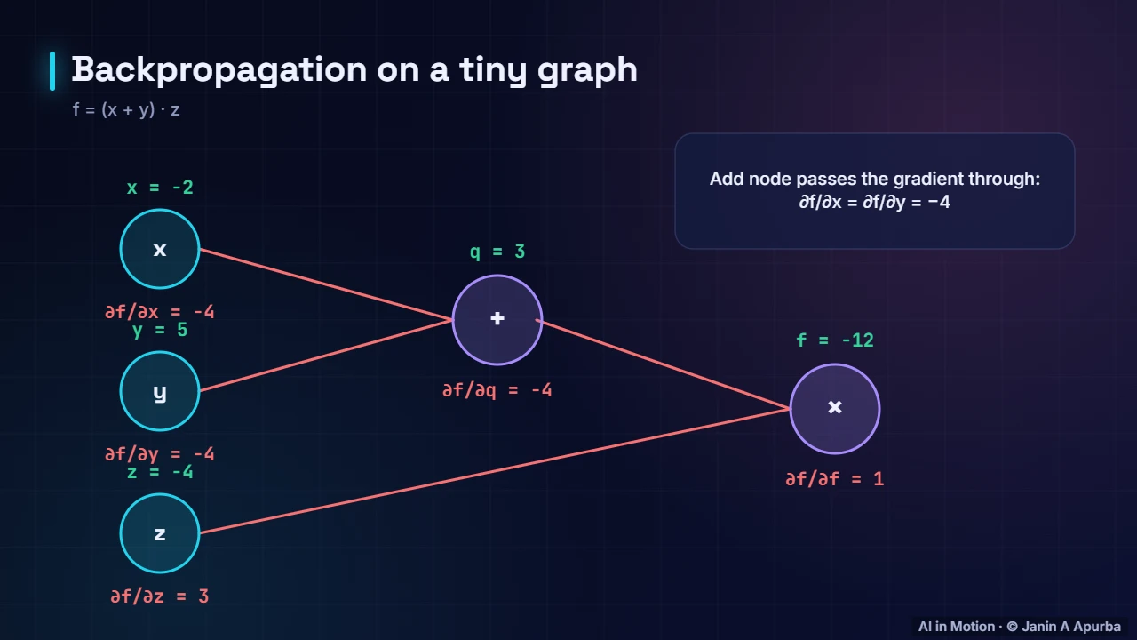
A tiny example. Take f equals x plus y, times z, with x equals minus 2, y equals 5 and z equals minus 4. Forward: q equals x plus y equals 3, and f equals q times z equals minus 12. Now backward. Start with a gradient of 1 at f. At the multiply node, the gradient for z is q, which is 3, and for q it is z, minus 4. The add node passes minus 4 to both x and y.
Chain rule. That is the chain rule. The gradient of f with respect to x equals the gradient of f with respect to q, times the gradient of q with respect to x. Minus four times one gives minus four. Backpropagation applies this rule node by node, from the output back to the inputs.
In a real network. In a real network it is the same idea at scale. The forward pass computes predictions and the loss. The backward pass sends error signals back through every layer, giving each weight a gradient. Then gradient descent updates them all.
Why it matters. Backpropagation is efficient. One backward pass gives every weight its gradient, at roughly the cost of a forward pass. Modern frameworks do it automatically, a feature called automatic differentiation.
Recap. To recap. Compute values forward. Apply the chain rule backward. Every weight gets a gradient. And gradient descent uses those gradients to improve the network.