Training Deep Neural Networks: A Practical Deep Dive — lecture notes
The full recipe for training a network well: forward pass, softmax and cross-entropy, backpropagation, initialisation, vanishing gradients and skip connections, normalisation, optimisers, regularisation and a debugging checklist.
0:001. Introduction
Designing a neural network is the easy part. Getting it to train well is where most of the craft lies. In this deep dive we walk through the complete recipe: the forward pass, the loss, backpropagation, initialisation, normalisation, optimisers, regularisation, and how to debug a network that refuses to learn.
0:212. What training means
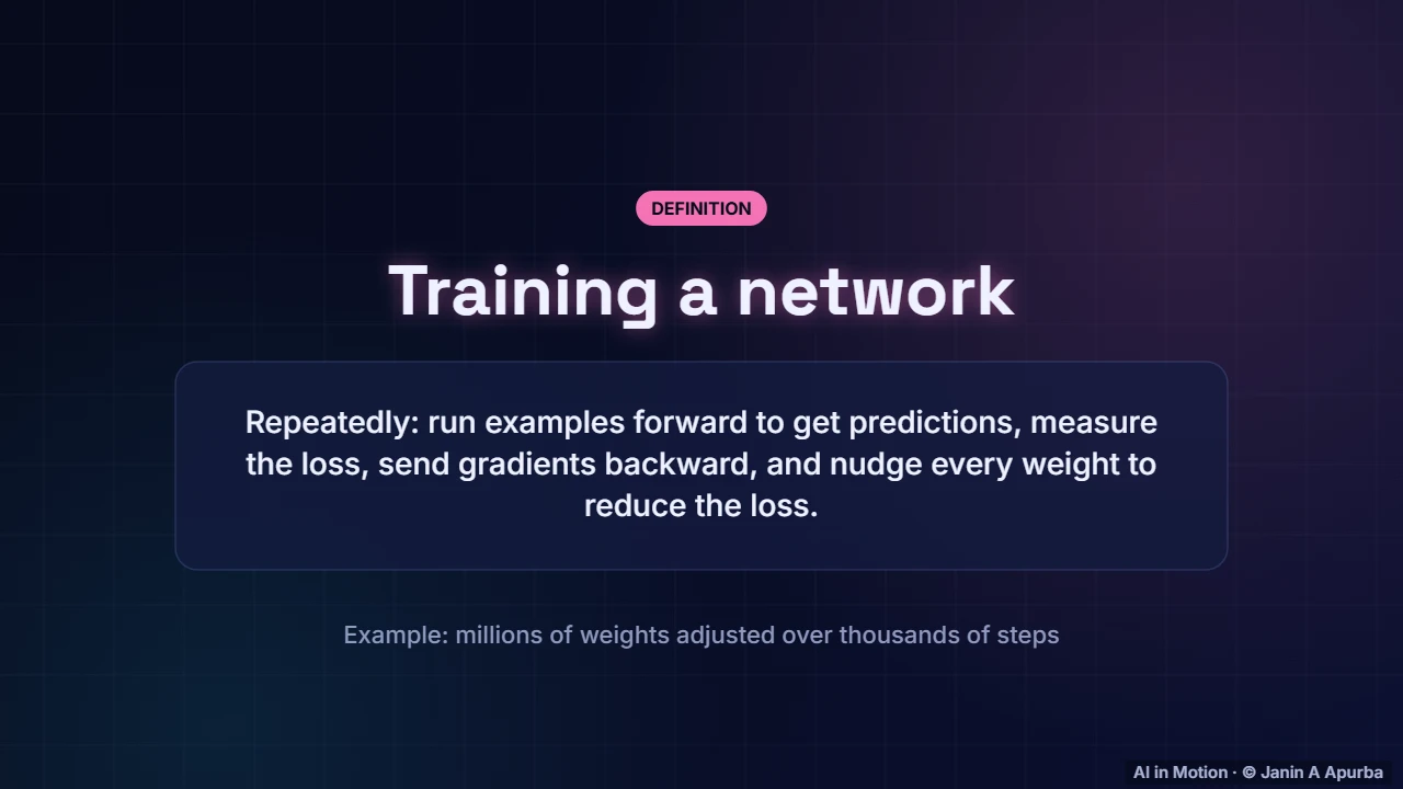
Training a network means repeating four steps. Run a batch of examples forward to get predictions, measure how wrong they are with a loss, send gradients backward to every weight, and nudge each weight to reduce the loss. Do this thousands of times, and millions of weights gradually organise themselves.
0:423. The forward pass
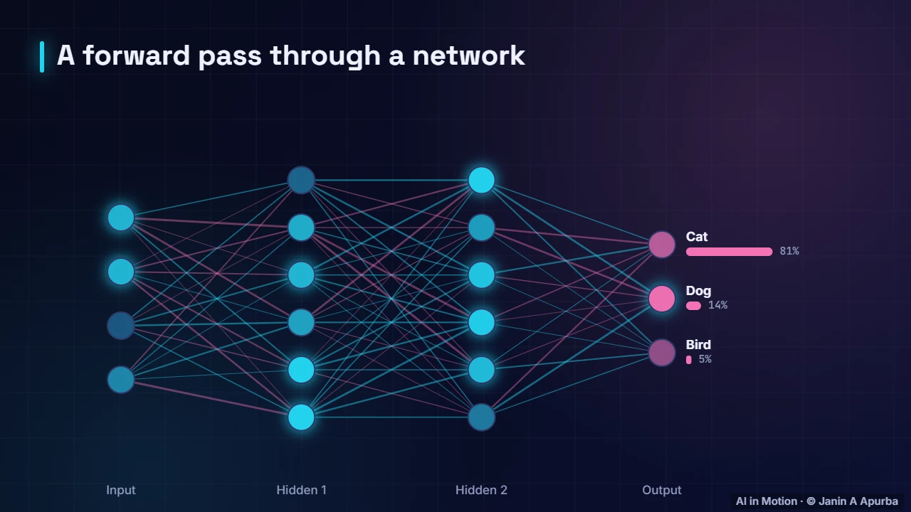
This network has four inputs, two hidden layers of six neurons and three outputs. In the forward pass, signals flow from left to right. Each neuron combines the signals from the previous layer, and the output layer produces probabilities: eighty one percent cat, fourteen percent dog, five percent bird.
1:034. Inside one neuron
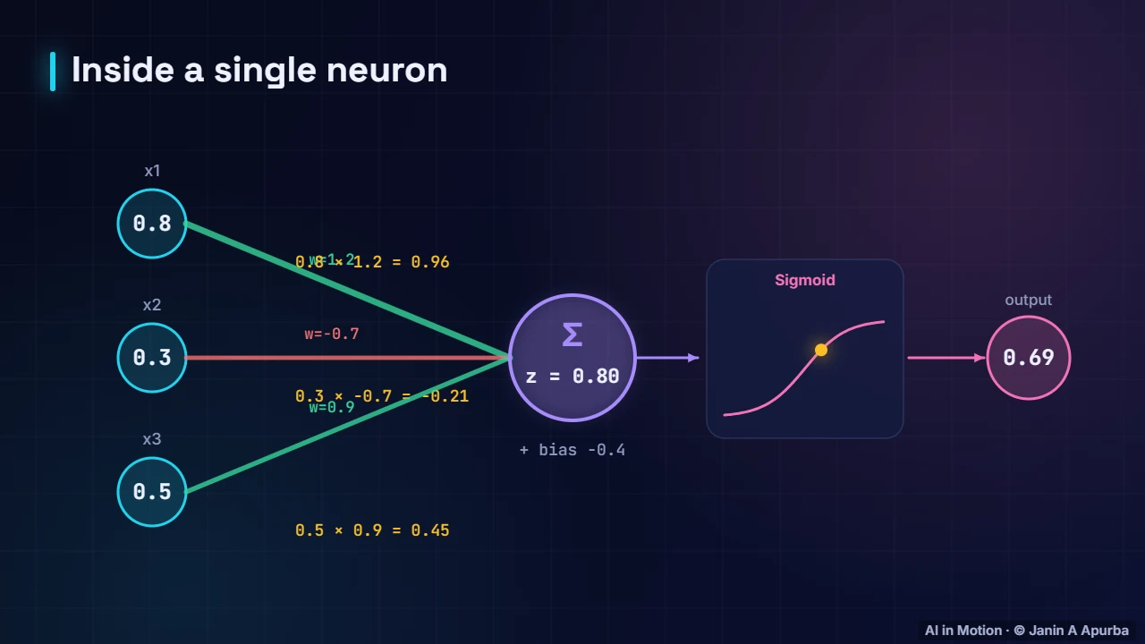
Zoom in on one neuron. Each input is multiplied by a weight: point eight times one point two, point three times minus point seven, and point five times point nine. Adding them with a bias of minus point four gives z equals point eight, and the sigmoid activation turns that into an output of about point six nine.
1:275. Activation functions
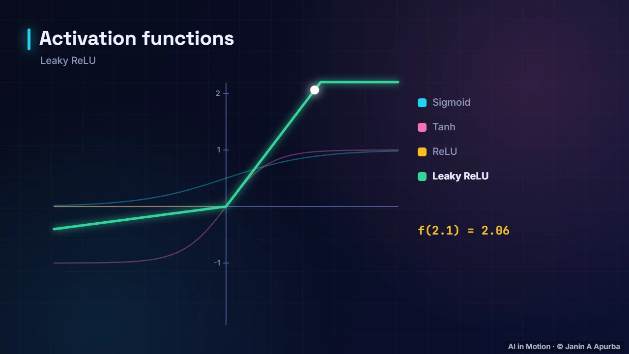
Activation functions give networks their power. The sigmoid squeezes values between zero and one, and tanh is similar but centred on zero. ReLU outputs zero for negatives and passes positives straight through. Leaky ReLU keeps a small slope for negatives, so neurons never die completely.
1:466. Pause and think
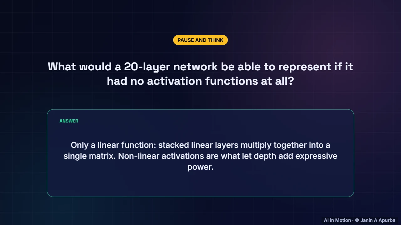
Pause and think. What could a twenty layer network represent if it had no activation functions at all? Only a linear function, because stacked linear layers multiply together into a single matrix. The non linear activations are what allow extra depth to add expressive power.
2:057. Softmax
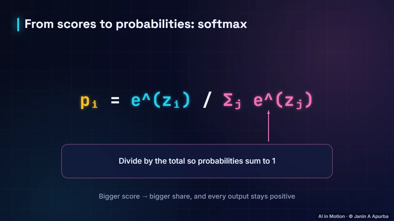
For classification, the final layer produces a score, or logit, for each class, and softmax turns scores into probabilities. It exponentiates every score, making them positive, and divides by their total, so the probabilities add up to one. Larger scores get larger shares.
2:248. Cross-entropy loss
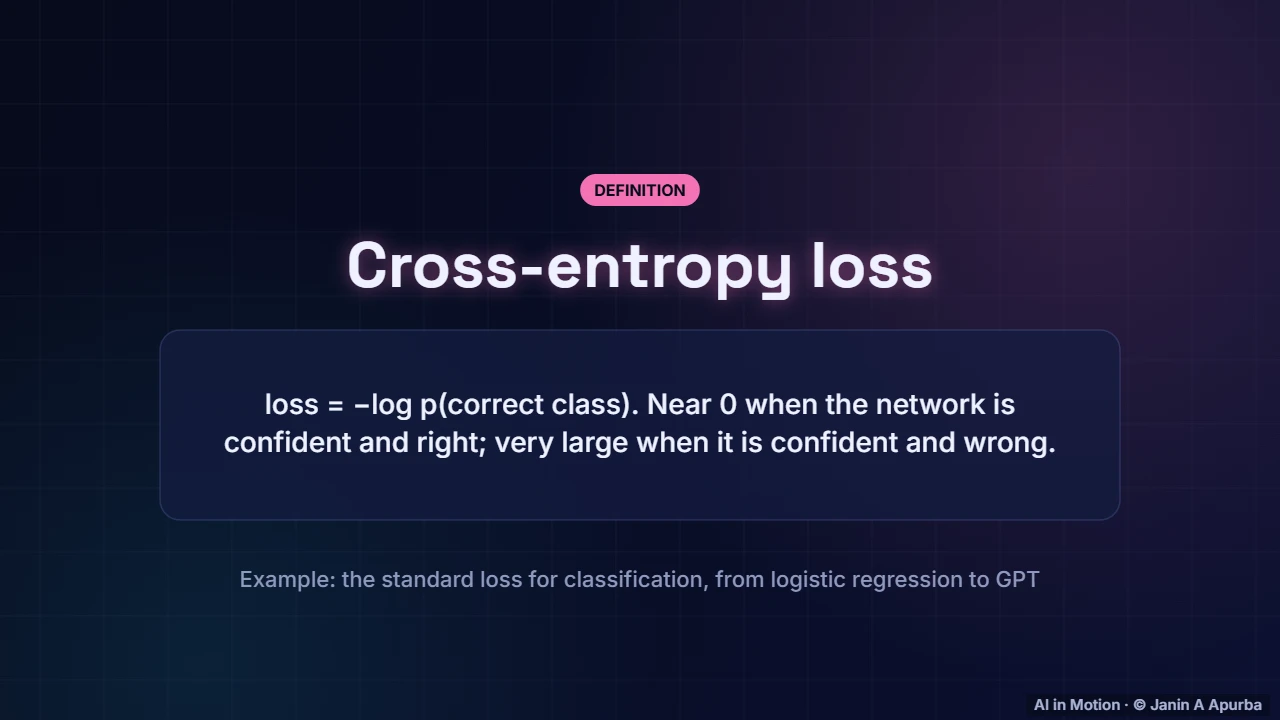
The standard classification loss is cross entropy: minus the log of the probability given to the correct class. If the network is confident and right, the loss is close to zero. If it is confident and wrong, the loss is very large, which pushes hard against overconfident mistakes.
2:449. Compute it
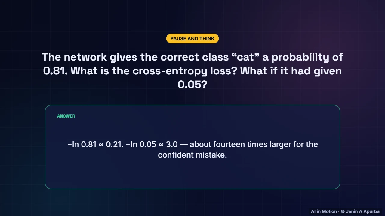
Let us compute it. The network gives the correct class, cat, a probability of point eight one. The loss is minus the natural log of point eight one, about point two one. Had it given only point zero five, the loss would be about three, fourteen times larger.
3:0510. Backpropagation
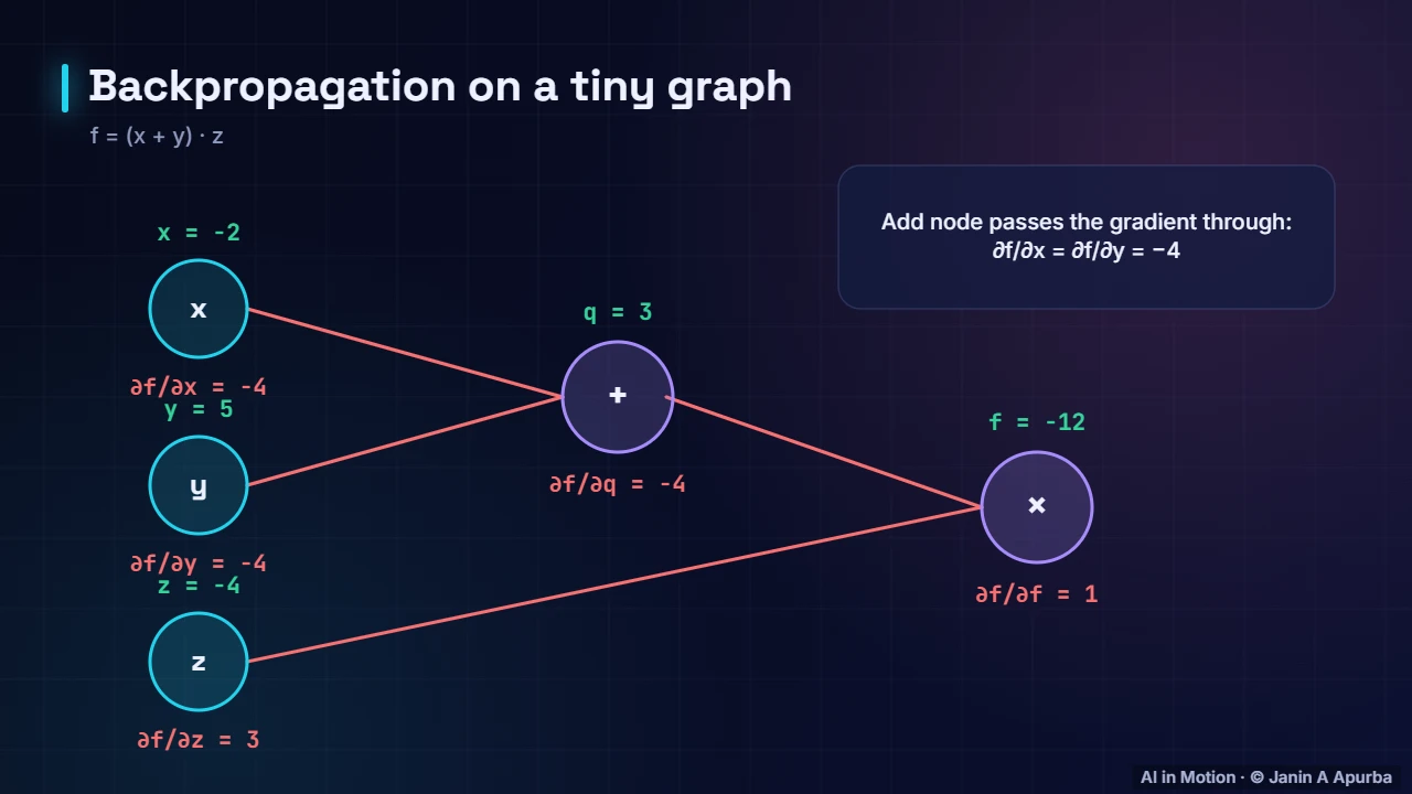
Backpropagation computes every gradient using the chain rule. Take f equals x plus y, times z, with x minus two, y five and z minus four. Forward, q is three and f is minus twelve. Backward, the gradient for z is q, three, and the gradient flowing to x and y is z, minus four.
3:2811. Forward and backward
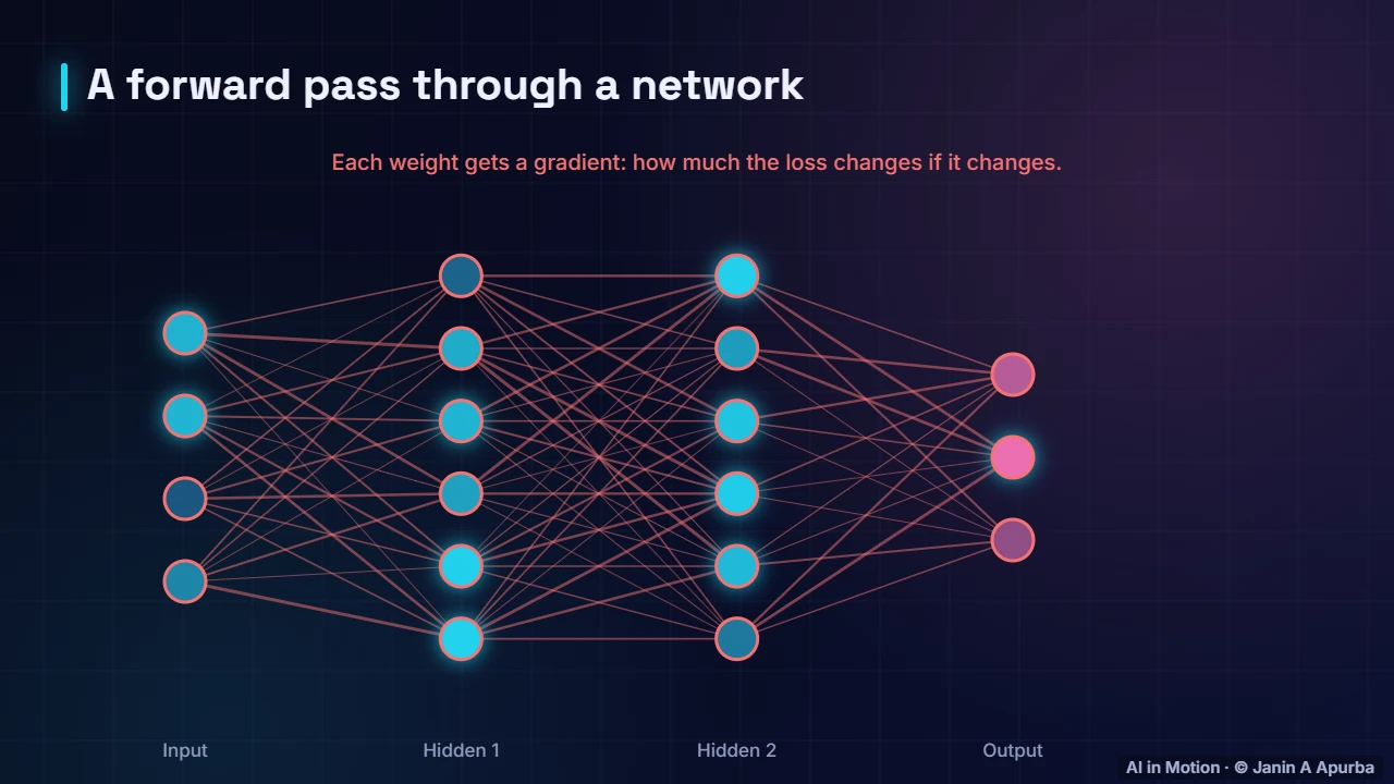
In a real network it is the same idea at scale. The forward pass computes predictions and the loss. The backward pass sends error signals back through every layer, giving each weight a gradient. Then the optimiser updates them all at once, and the next batch begins.
3:4812. Initialisation
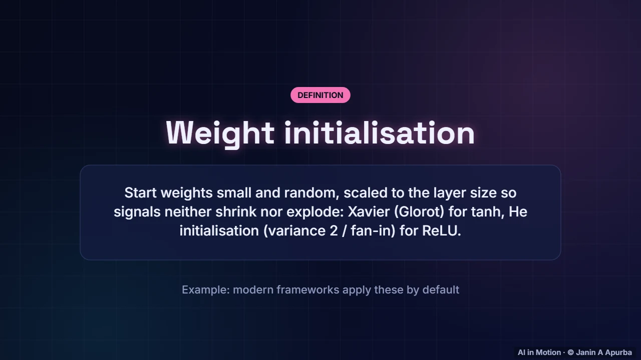
How weights start matters. They must be random, and scaled to the size of each layer so that signals neither shrink nor explode as they pass through many layers. Xavier initialisation suits tanh networks, and He initialisation, with variance two over the number of inputs, suits ReLU networks.
4:0813. Pause and think
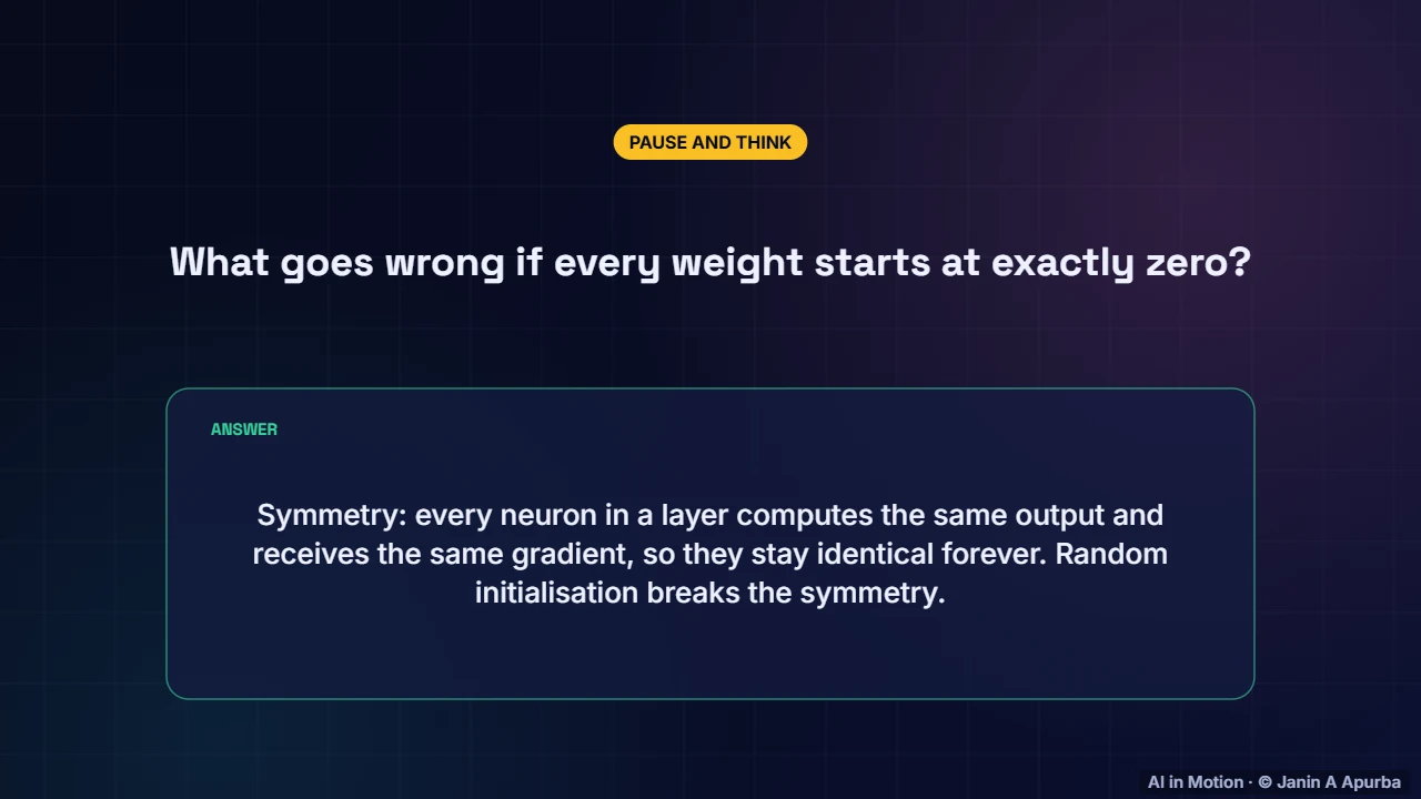
Pause and think. What goes wrong if every weight starts at exactly zero? All the neurons in a layer compute the same output and receive the same gradient, so they stay identical forever and the layer behaves like a single neuron. Random initialisation breaks this symmetry.
4:2814. Vanishing gradients
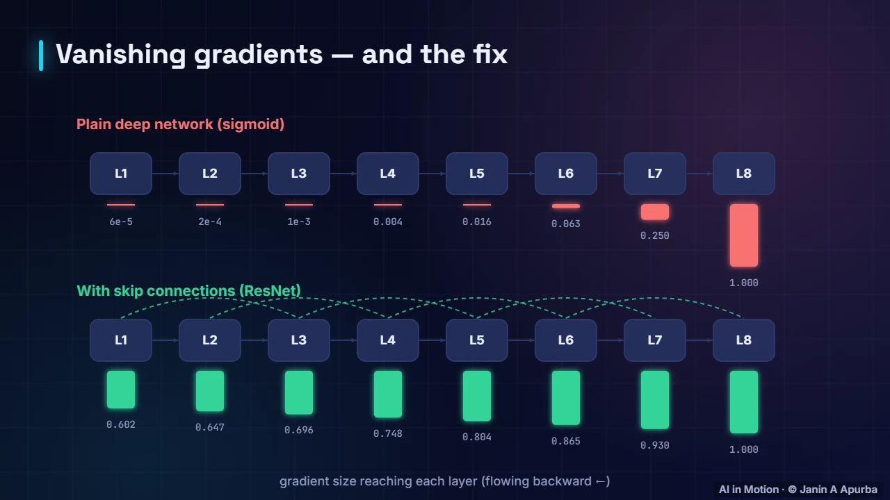
During backpropagation, the gradient is multiplied by each layer’s local slope on its way back. The sigmoid’s slope is at most point two five. Multiply by point two five again and again, and by the first of eight layers only about six hundred thousandths remain. Early layers barely learn.
4:4915. Skip connections
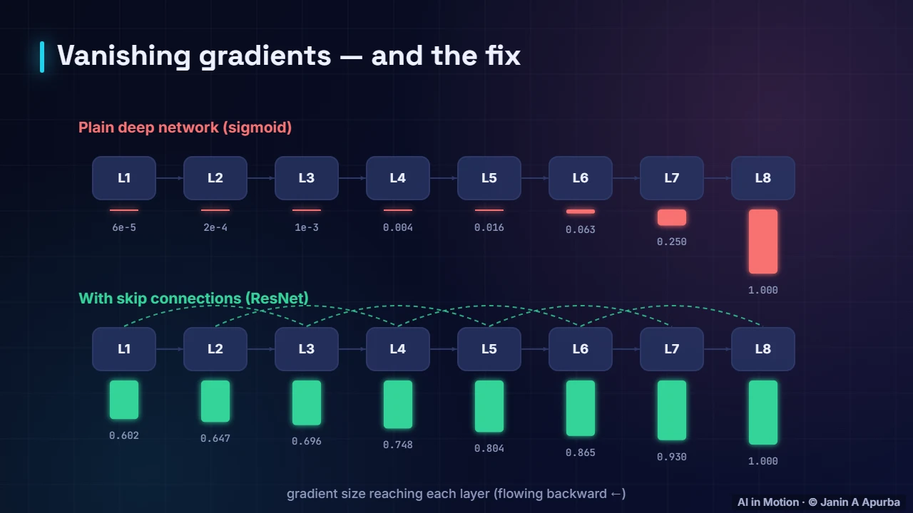
Residual networks add skip connections: each block adds its input to its output, giving the gradient a direct highway back through the network. In this illustration it stays around point six even at the first layer. This idea, from ResNet in 2015, made networks with over a hundred layers trainable.
5:1016. Normalisation
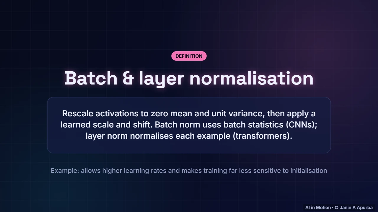
Normalisation layers keep activations well behaved. Batch normalisation rescales each feature using statistics of the current mini batch, and is common in convolutional networks. Layer normalisation normalises each example on its own, and is standard in transformers. Both allow higher learning rates and much more stable training.
5:3017. Optimisers
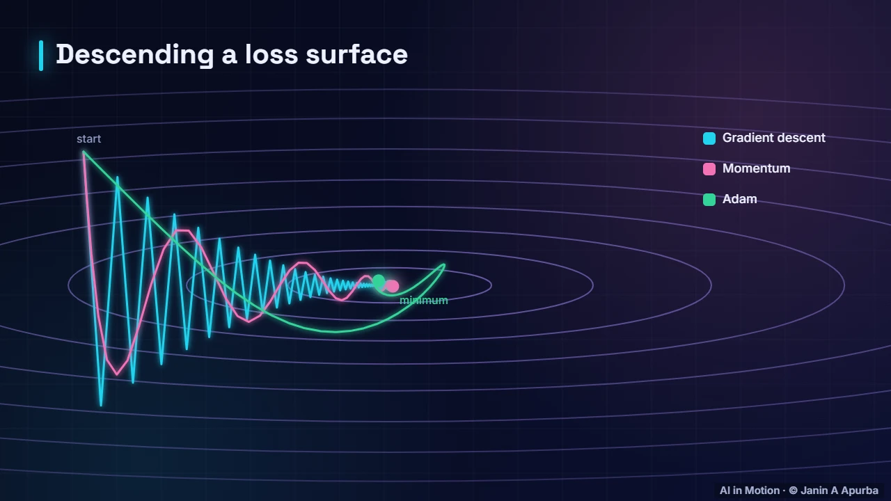
The optimiser decides how gradients become updates. On this narrow valley, plain gradient descent zig zags, Adam adapts its step size for each direction and heads almost straight in, and momentum builds up speed along the valley. For most networks, Adam or AdamW is a strong default.
5:5018. Learning-rate schedule
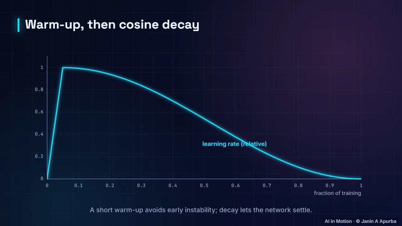
The learning rate usually follows a schedule. A short warm up starts small, avoiding chaotic early updates while the weights are still random. Then the rate decays, here along a cosine curve, so that late training takes small, careful steps and the network settles into a good solution.
6:1019. The training loop
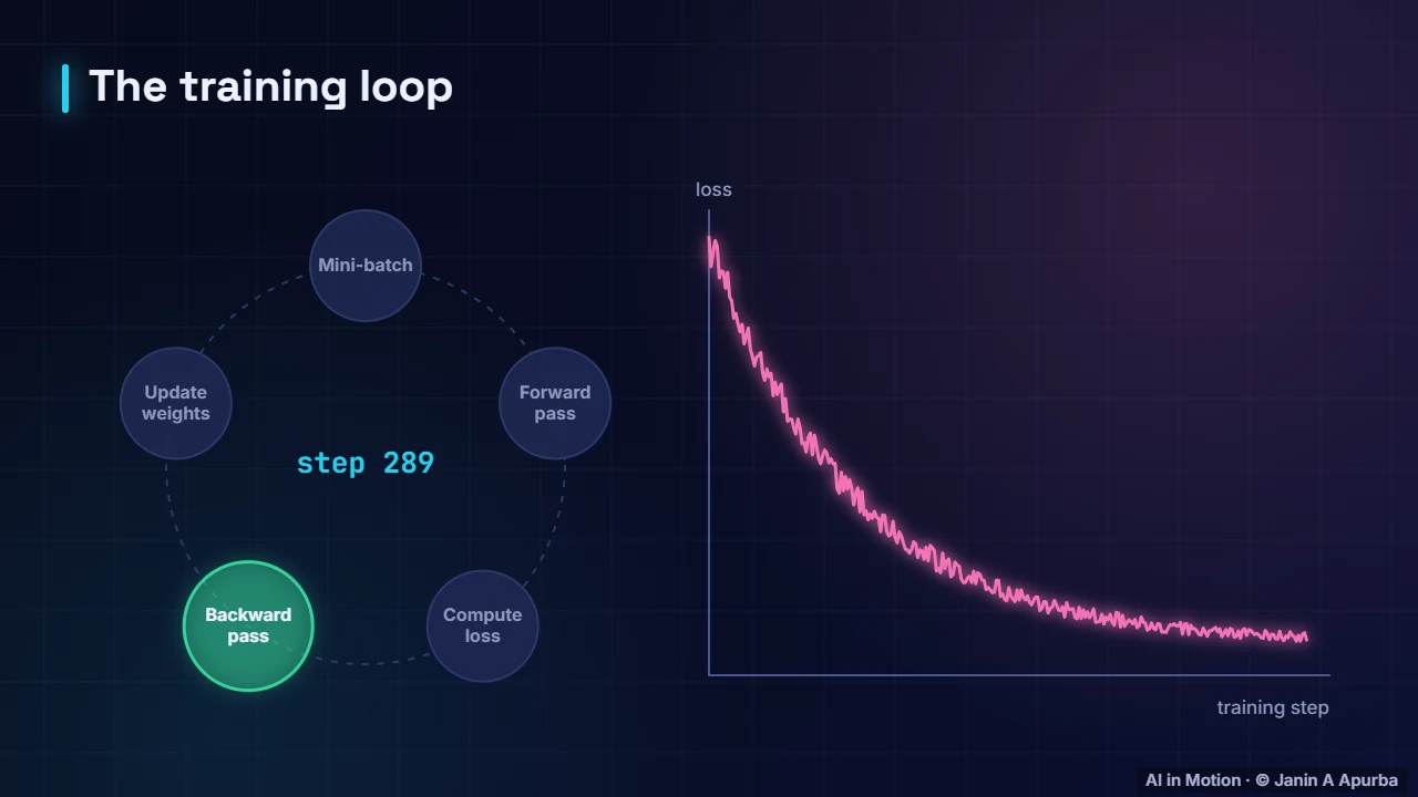
Here is the loop in action. Take a mini batch of examples. Run a forward pass to get predictions. Compute the loss. Run a backward pass to find how each weight affects the loss. Update the weights a little. Then take the next batch. The loss on the right falls as training goes on.
6:3320. Overfitting
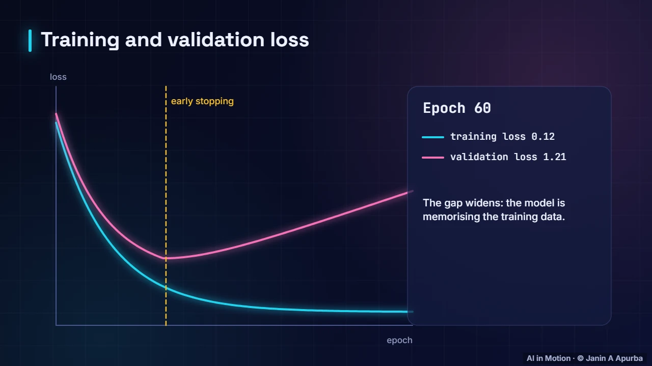
Deep networks have enough capacity to memorise their training data. Learning curves reveal it: training loss keeps falling, but validation loss stops improving and starts to rise. The widening gap means the model is memorising rather than learning patterns that generalise.
6:5121. Regularisation
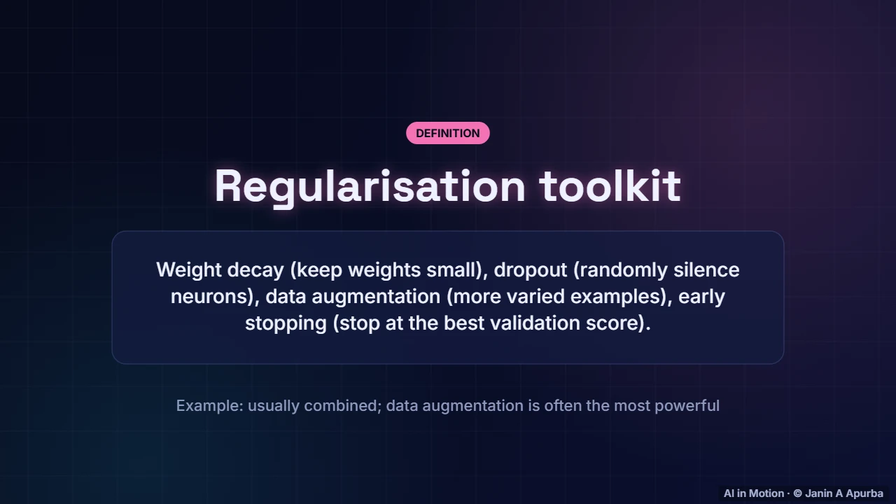
Regularisation fights overfitting. Weight decay keeps weights small. Dropout randomly silences neurons. Data augmentation creates varied versions of each training example. Early stopping halts training at the best validation score. They are usually combined, and more real data beats them all.
7:0822. Dropout
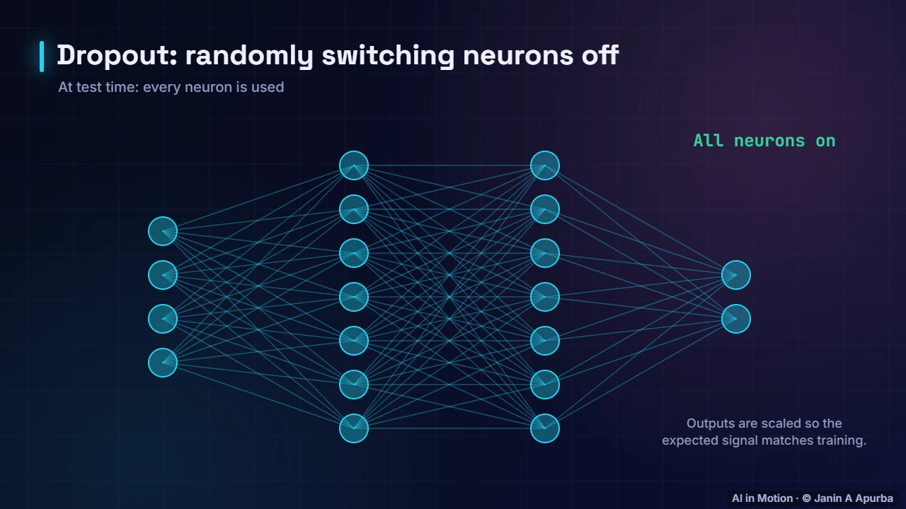
Dropout randomly switches off about half of the hidden neurons at every training step, a different random set each time. No neuron can rely on a particular partner, so the network learns more robust, spread out features. At test time, every neuron is used, with outputs scaled to match.
7:2923. Data augmentation
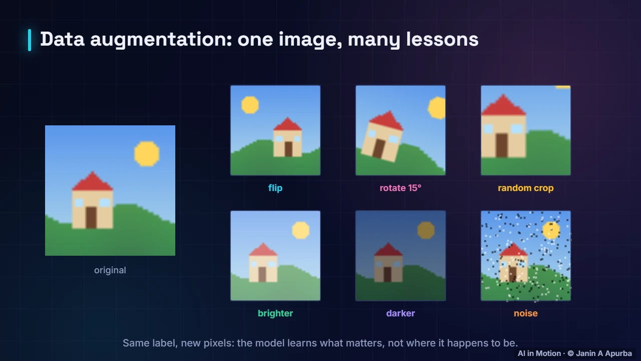
For images, data augmentation is especially powerful. Take one image and flip it, rotate it slightly, crop it, change its brightness or add a little noise. The label stays the same, so the network learns that these changes do not matter, and it sees far more variety than the raw dataset contains.
7:5124. A healthy run
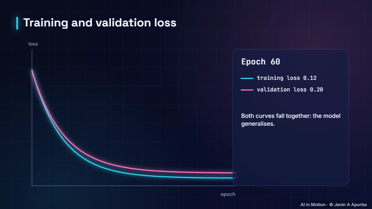
With the right regularisation, training and validation loss fall together and stay close. That is the signature of a network that is genuinely learning. If both curves stay high instead, the model is underfitting and needs more capacity, better features or longer training.
8:1025. Start small
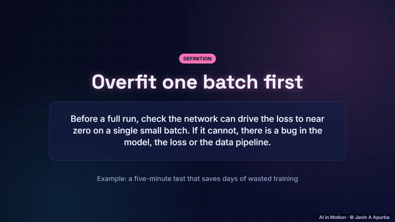
A wise first step in any project is to overfit one small batch. A healthy network should be able to memorise a handful of examples, driving the loss close to zero. If it cannot, there is a bug in the model, the loss or the data pipeline. This five minute test can save days.
8:3226. Troubleshooting
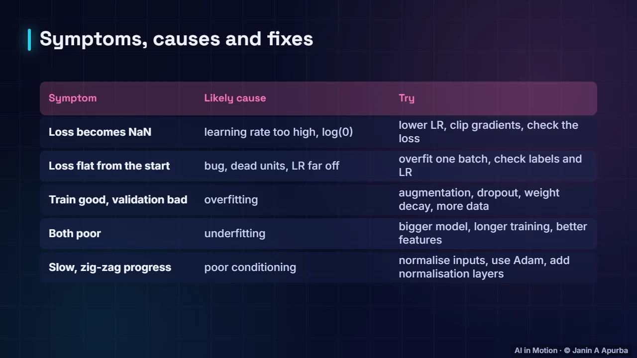
Here is a troubleshooting table. A loss that becomes not a number usually means the learning rate is too high. A flat loss from the start suggests a bug. Good training but poor validation is overfitting. Poor results on both mean underfitting, and slow zig zag progress calls for normalisation and adaptive optimisers.
8:5527. Pause and think
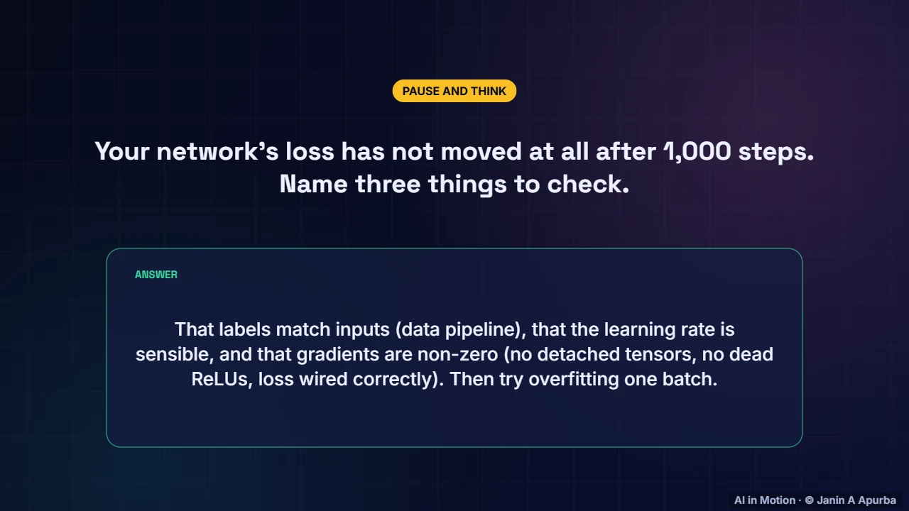
Pause and think. Your loss has not moved at all after a thousand steps. What should you check? That the labels actually match the inputs, that the learning rate is sensible, and that gradients are flowing and non zero. Then try to overfit a single batch to isolate the problem.
9:1628. Memory and precision
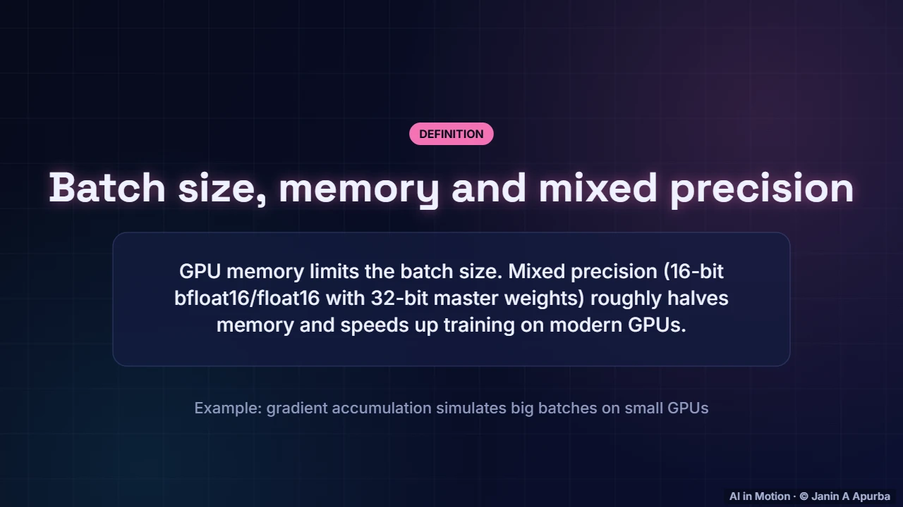
GPU memory limits how large a batch can be. Mixed precision training computes in sixteen bit numbers while keeping a thirty two bit master copy of the weights, roughly halving memory and speeding up modern GPUs. Gradient accumulation sums gradients over several small batches to simulate a large one.
9:3729. In code
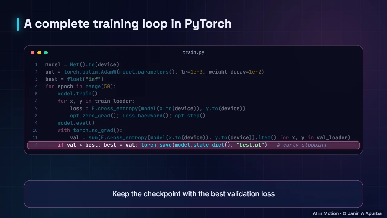
Here is a complete loop in PyTorch. Put the model on the GPU and create an AdamW optimiser. In training mode, run forward, compute cross entropy, backpropagate and step. Then switch to evaluation mode, which changes dropout and batch norm behaviour, measure validation loss without gradients, and keep the best checkpoint.
9:5830. Do not start from scratch
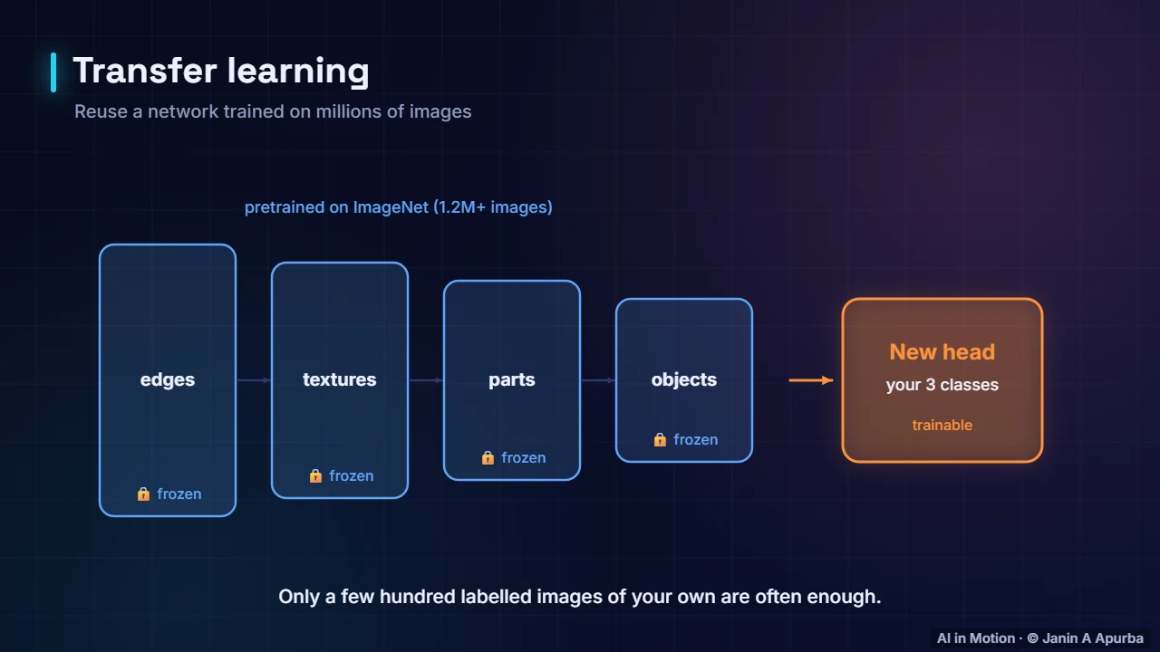
Finally, you rarely need to train from scratch. Take a network pre trained on a huge dataset, such as ImageNet with over a million images. Its layers already detect edges, textures and parts. Freeze them, add a new head for your classes and train only that, with far less data and time.
10:2031. A training recipe
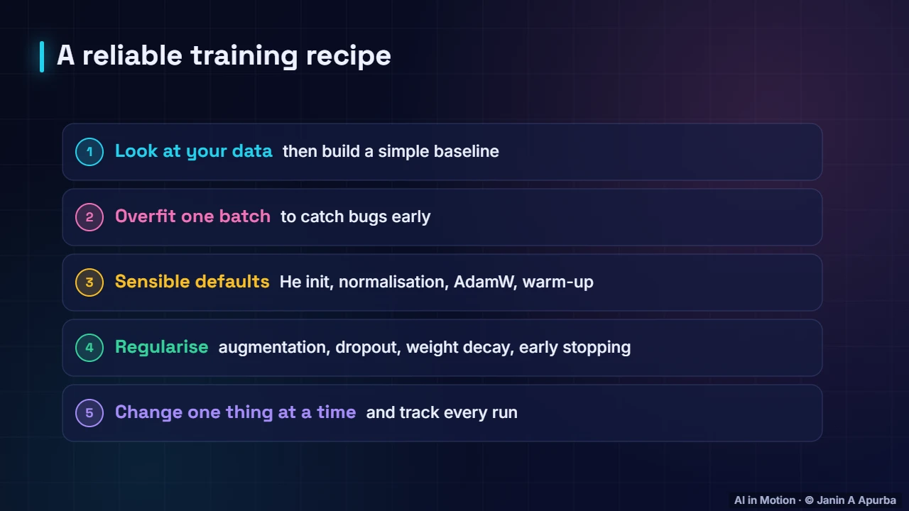
Here is a reliable recipe. Look closely at your data and build a simple baseline. Overfit one batch to catch bugs. Start from sensible defaults: He initialisation, normalisation layers, AdamW with warm up. Add regularisation as needed, change one thing at a time, and track every experiment.
10:4132. Recap
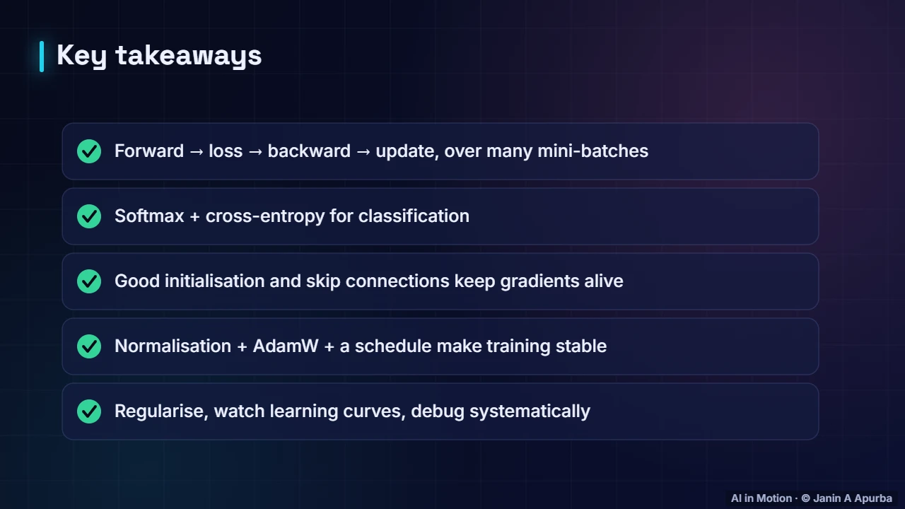
To recap. Training repeats forward, loss, backward and update over many mini batches, with softmax and cross entropy for classification. Good initialisation and skip connections keep gradients alive. Normalisation, AdamW and a schedule make training stable, and regularisation plus systematic debugging get you to a model that generalises.
Key takeaways
- Training repeats forward pass → loss → backpropagation → optimiser update over mini-batches.
- Softmax turns logits into probabilities; cross-entropy (−log p of the correct class) punishes confident mistakes.
- Random, size-scaled initialisation (Xavier/He) breaks symmetry and keeps signals stable.
- Vanishing gradients in deep sigmoid networks are eased by ReLU, normalisation and residual skip connections.
- Regularise with weight decay, dropout, data augmentation and early stopping; watch training vs validation curves.
- Debug by overfitting one batch first, then change one thing at a time.
Check yourself
- What does softmax guarantee about its outputs?
Show answer
They are positive and sum to 1 — Exponentiate, then normalise.
- Cross-entropy loss when the correct class gets probability 0.81 is about…
Show answer
0.21 — −ln 0.81 ≈ 0.21.
- Why not initialise all weights to zero?
Show answer
All neurons would stay identical (symmetry) — Identical neurons get identical gradients.
- What problem do residual (skip) connections mainly address?
Show answer
Vanishing gradients in very deep networks — They give gradients a direct path back.
- A useful first debugging step for a new network is to…
Show answer
Overfit a single small batch — If it cannot memorise a batch, there is a bug.
Go deeper
- Debugging Neural Network Training: A Systematic Recipe · The AI Lecture Hall
- Weight Initialisation: Xavier, He and Why It Matters · The AI Lecture Hall
- Batch Normalisation: Faster, More Stable Training · The AI Lecture Hall
- Regularisation in Deep Learning: Weight Decay, Early Stopping, Augmentation and More · The AI Lecture Hall
- Loss Functions in Deep Learning: What Are We Really Optimising? · The AI Lecture Hall
© 2026 Janin A Apurba, CSE, AUST · Advanced ICT Officer, CNRS-UNHCR. All rights reserved. Notes for the animated lecture at https://ai-in-motion.vercel.app/watch/training-deep-networks-deep-dive.html