Large Language ModelsDeep diveAdvanced11:09 video31 chapters

Pre-training LLMs at Scale — lecture notes

The recipe behind base models: web-scale data pipelines, next-token loss and perplexity, scaling laws and compute budgets, Chinchilla, distributed training, learning-rate schedules and what can go wrong.

▶ Watch the animated lecture

0:001. Introduction

Introduction — Pre-training LLMs at Scale

Before a language model can chat, it must be pre trained: shown trillions of tokens of text and asked, again and again, to predict what comes next. This deep dive covers the recipe behind that expensive first stage: the data, the objective, the scaling laws and the engineering that holds it together.

0:212. Self-supervised learning

Self-supervised learning — Pre-training LLMs at Scale

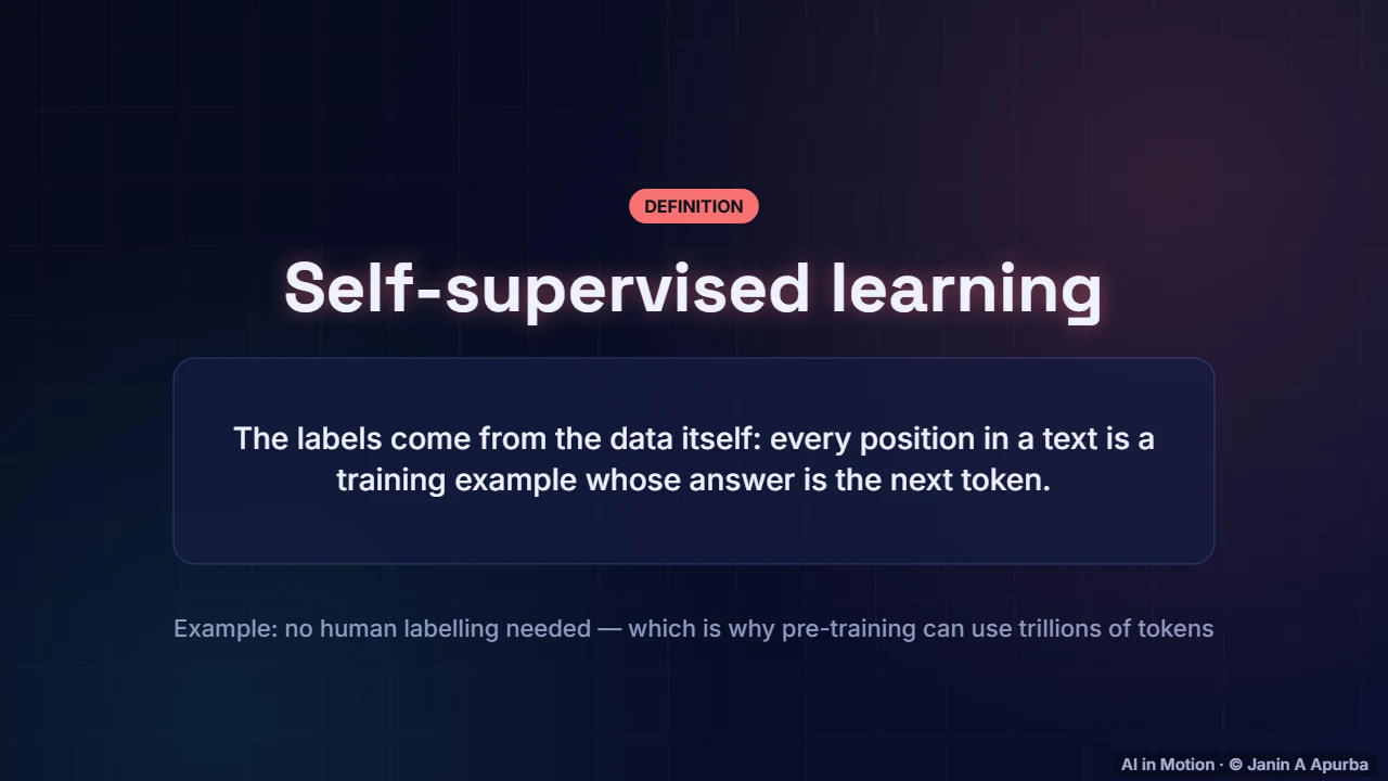
Pre training is self supervised. Nobody labels anything: the text supplies its own answers, because every position’s target is simply the next token. That is why pre training can use trillions of tokens. The internet, books and code become an enormous set of fill in the next word exercises.

0:423. The objective

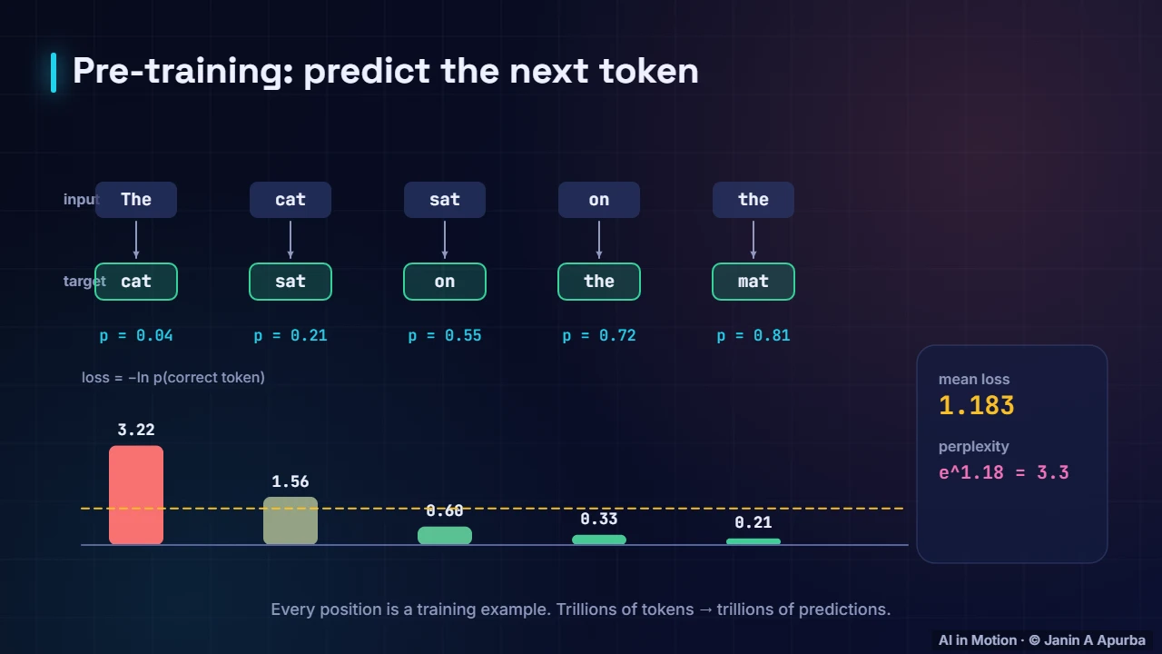
The objective — Pre-training LLMs at Scale

Here is the objective on a tiny sentence. The inputs are the tokens, and the targets are the same tokens shifted by one. At each position the model assigns a probability to the correct next token, and the loss is minus its logarithm. Averaged here, the loss is about one point one eight, a perplexity of about three point three.

1:064. Training the tokenizer first

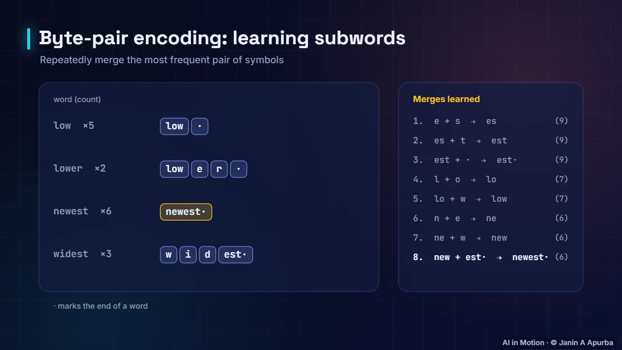
Training the tokenizer first — Pre-training LLMs at Scale

Before pre training begins, a tokenizer is trained on a sample of the data, usually with byte pair encoding. It repeatedly merges the most frequent pairs of symbols into new tokens. Its vocabulary, often thirty two thousand to over a hundred thousand tokens, is fixed for the model’s whole life, so it is chosen carefully.

1:295. Loss and perplexity

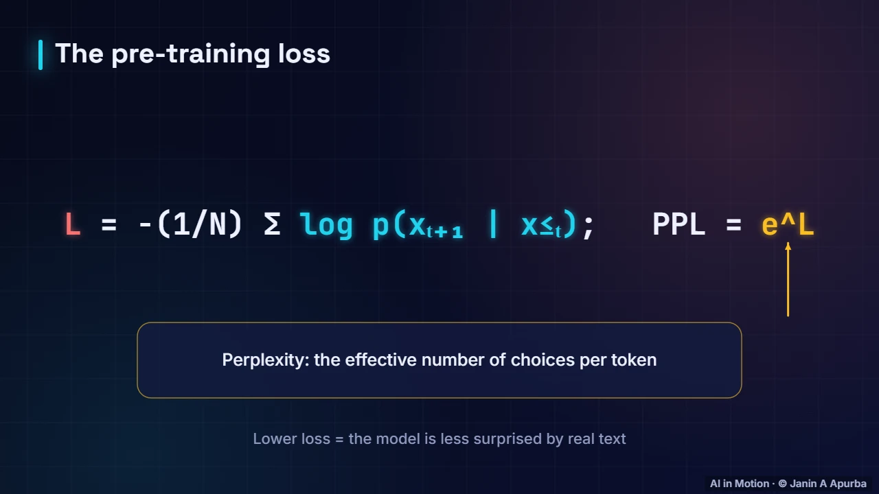
Loss and perplexity — Pre-training LLMs at Scale

Formally, the loss is the average negative log probability of each real next token, which is the cross entropy between the data and the model. Its exponential is the perplexity, roughly how many equally likely choices the model is torn between. Lower loss means the model is less surprised by real text.

1:516. The data pipeline

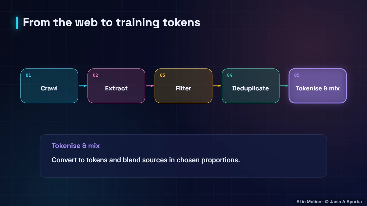
The data pipeline — Pre-training LLMs at Scale

Most of the work is data. Pipelines start from web crawls such as Common Crawl, plus books, code and papers. Text is extracted from HTML, then filtered by language, quality and safety, with personal information removed. Near duplicate documents are removed, and the sources are tokenised and blended in chosen proportions.

2:137. Data scale

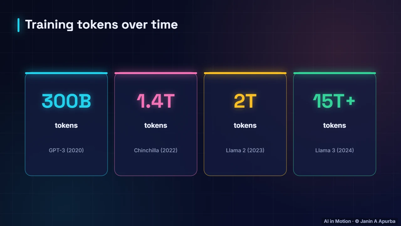
Training sets have grown fast. GPT three was trained on about three hundred billion tokens. Chinchilla used one point four trillion, Llama two used two trillion, and Llama three more than fifteen trillion. For comparison, a person reading all day for a lifetime encounters perhaps a billion words.

2:338. Data mixture

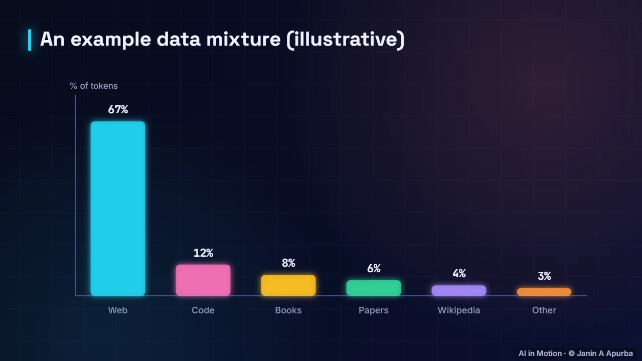
Data mixture — Pre-training LLMs at Scale

The mixture matters. A typical recipe is mostly filtered web text, with meaningful shares of code, books, scientific papers and encyclopedic text. Code improves reasoning and programming ability, and high quality sources are often sampled more than once. Getting the mixture right is a closely guarded part of every lab’s recipe.

2:559. Pause and think

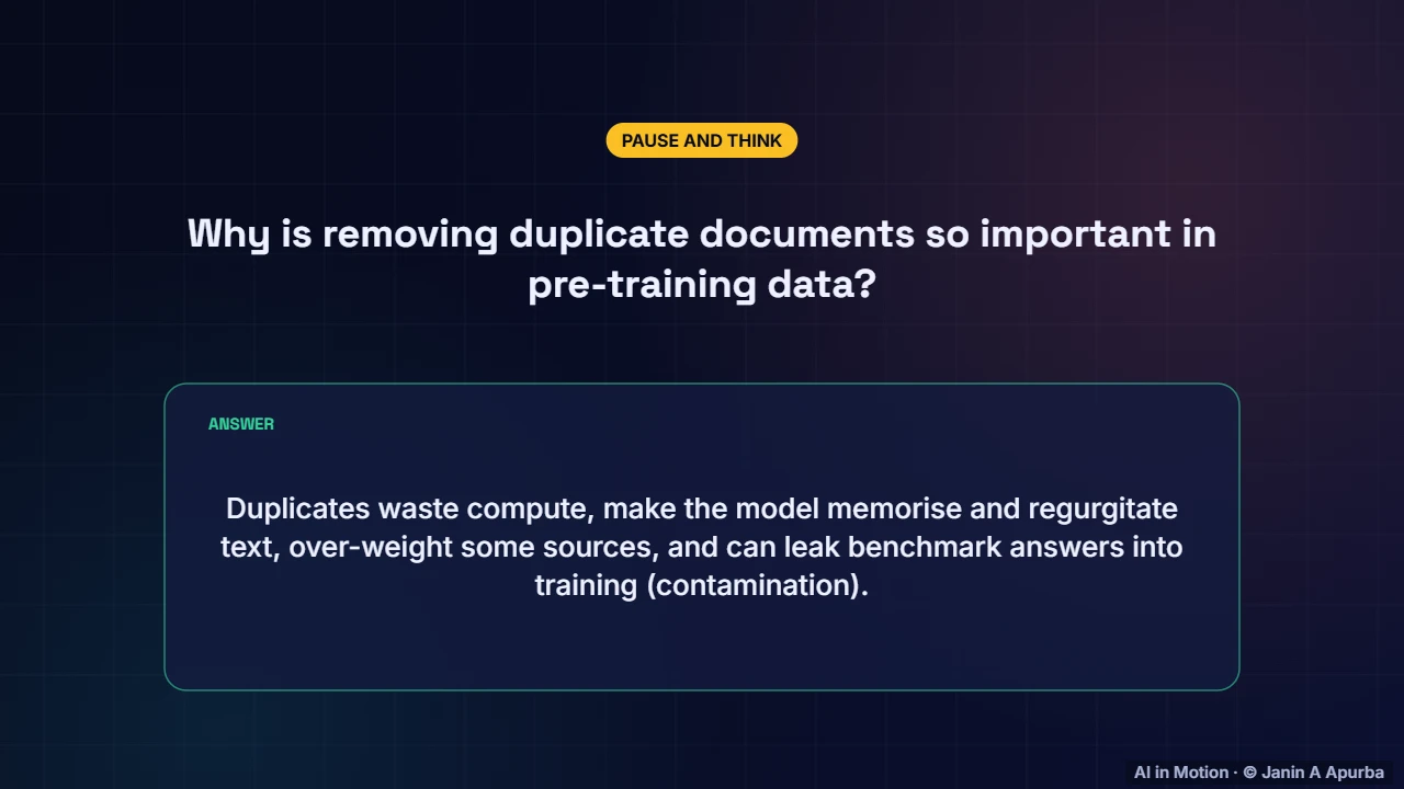
Pause and think — Pre-training LLMs at Scale

Pause and think. Why is removing duplicate documents so important? Duplicates waste compute, encourage the model to memorise and repeat text word for word, over weight some sources, and can leak evaluation questions into training, which makes benchmark scores misleadingly high.

3:1310. Synthetic data

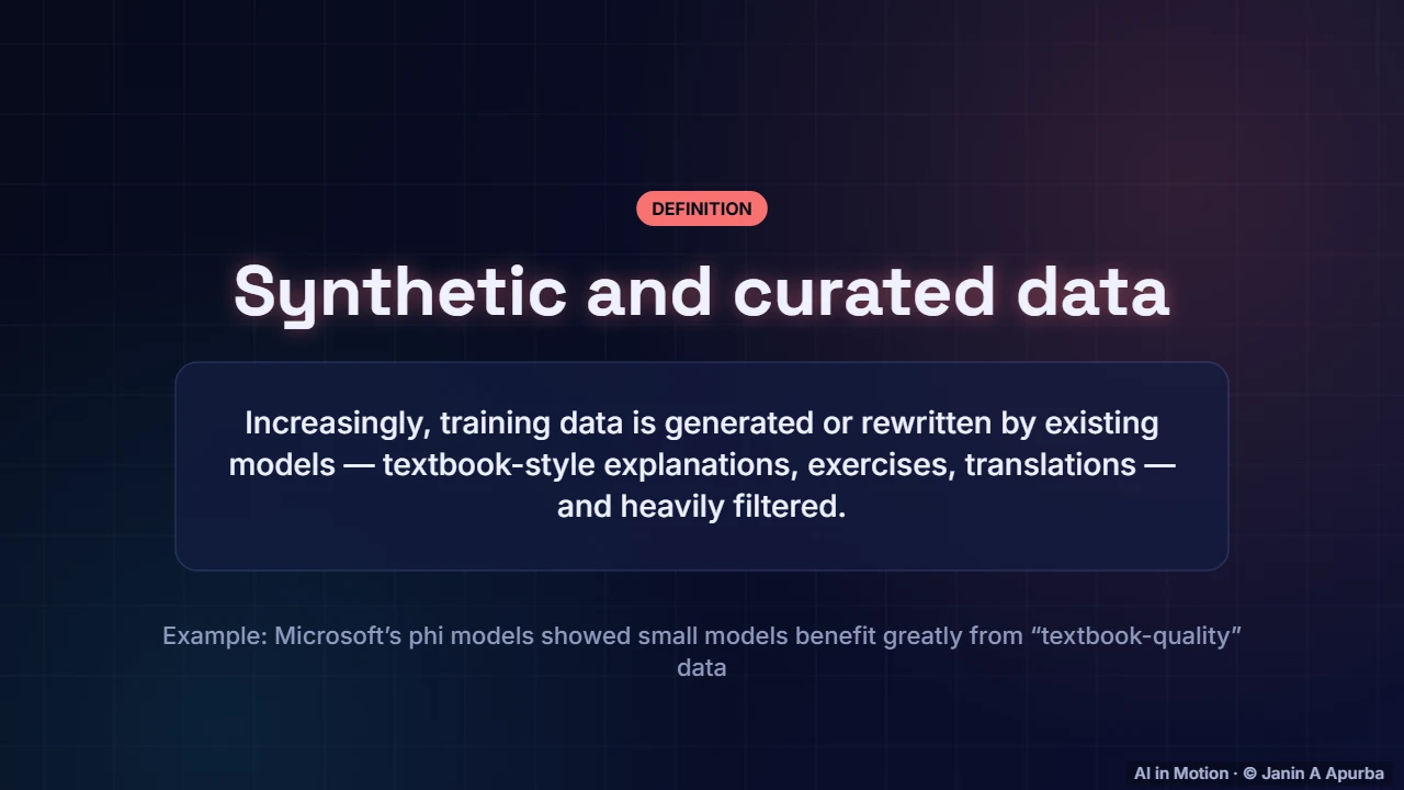
Synthetic data — Pre-training LLMs at Scale

Increasingly, training data is also synthetic: generated or rewritten by existing models as textbook style explanations, exercises and dialogues, then heavily filtered. Microsoft’s phi models showed that small models can benefit greatly from such textbook quality data. The risk is amplifying the mistakes and biases of the generating model.

3:3411. Batches of tokens

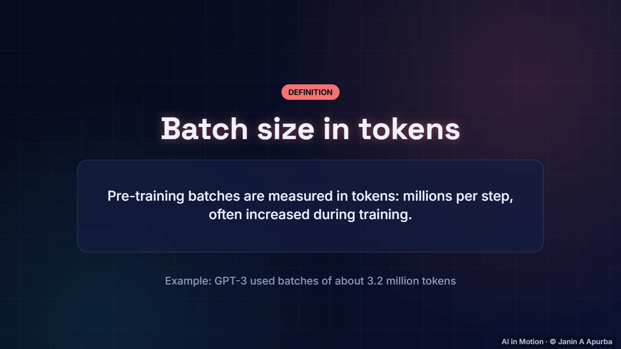
Batches of tokens — Pre-training LLMs at Scale

Batches in pre training are measured in tokens, not examples, and they are huge: millions of tokens per optimisation step. GPT three used batches of about three point two million tokens. Very large batches give smooth, stable gradients and keep thousands of GPUs busy in parallel.

3:5312. Scaling laws

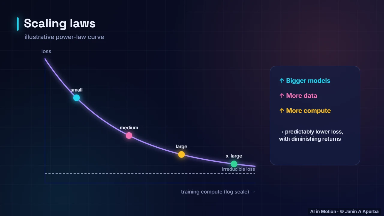
Scaling laws — Pre-training LLMs at Scale

In 2020, researchers discovered scaling laws: the loss falls smoothly and predictably, as a power law, when you increase parameters, data or compute. Plotted on log scales these are nearly straight lines. That predictability let labs forecast the performance of huge models from small experiments before spending millions.

4:1413. The compute budget

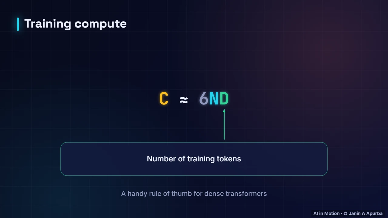
The compute budget — Pre-training LLMs at Scale

A handy rule of thumb gives the training compute: about six times the number of parameters times the number of training tokens. Two of those operations per parameter per token come from the forward pass and four from the backward pass. It lets you estimate the cost of any training run on the back of an envelope.

4:3814. Pause and think

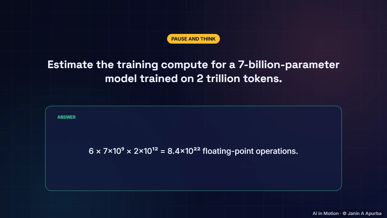
Let us use it. Estimate the compute for a seven billion parameter model trained on two trillion tokens. Six times seven billion times two trillion gives about eight point four times ten to the twenty two floating point operations, an enormous number that takes thousands of GPUs weeks to deliver.

4:5915. Chinchilla

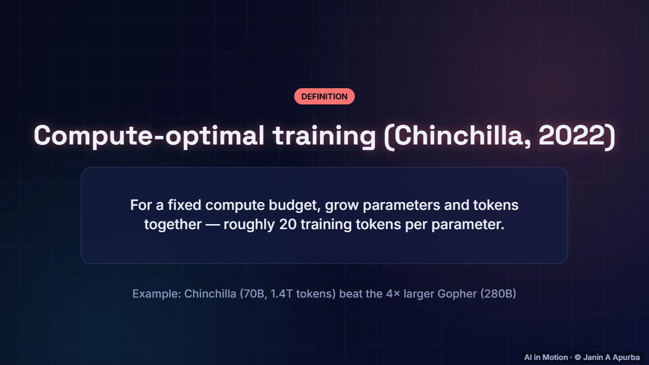
How should a fixed budget be split between model size and data? The 2022 Chinchilla study found that earlier models were too big for their data. The compute optimal ratio is roughly twenty tokens per parameter. Chinchilla, with seventy billion parameters and one point four trillion tokens, beat a four times larger model.

5:2116. Pause and think

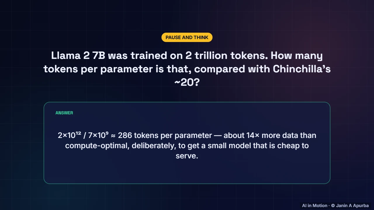
Pause and think. Llama two seven B saw two trillion tokens. How many tokens per parameter is that? Two trillion divided by seven billion is about two hundred and eighty six, roughly fourteen times the Chinchilla ratio. That was deliberate: extra training for a small model that is cheap to serve.

5:4317. Beyond compute-optimal

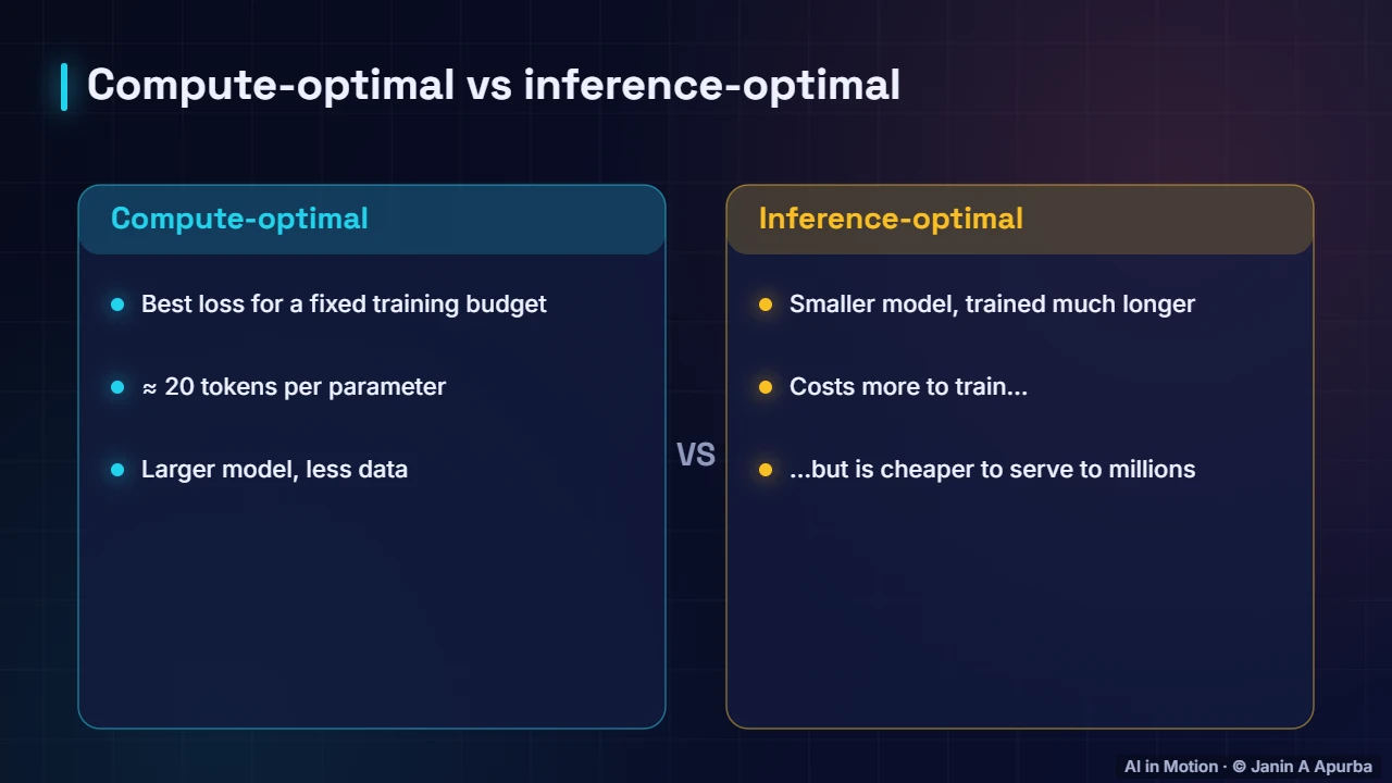
Beyond compute-optimal — Pre-training LLMs at Scale

But training cost is not the whole story. A model that will serve millions of users should be small and cheap to run. So many labs deliberately train smaller models on far more than twenty tokens per parameter. Llama models did exactly this, trading extra training compute for cheaper, faster inference.

6:0418. Mixed precision

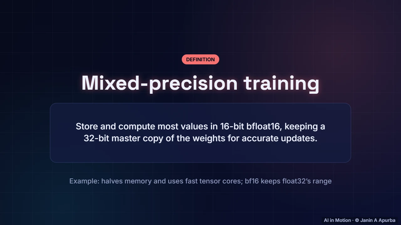
Mixed precision — Pre-training LLMs at Scale

Training at this scale uses mixed precision. Most computation happens in sixteen bit bfloat16 numbers, which halves memory and uses fast tensor cores on modern GPUs, while a thirty two bit master copy of the weights keeps updates accurate. Bfloat16 keeps the same range as thirty two bit floats, which avoids overflow.

6:2619. Distributed training

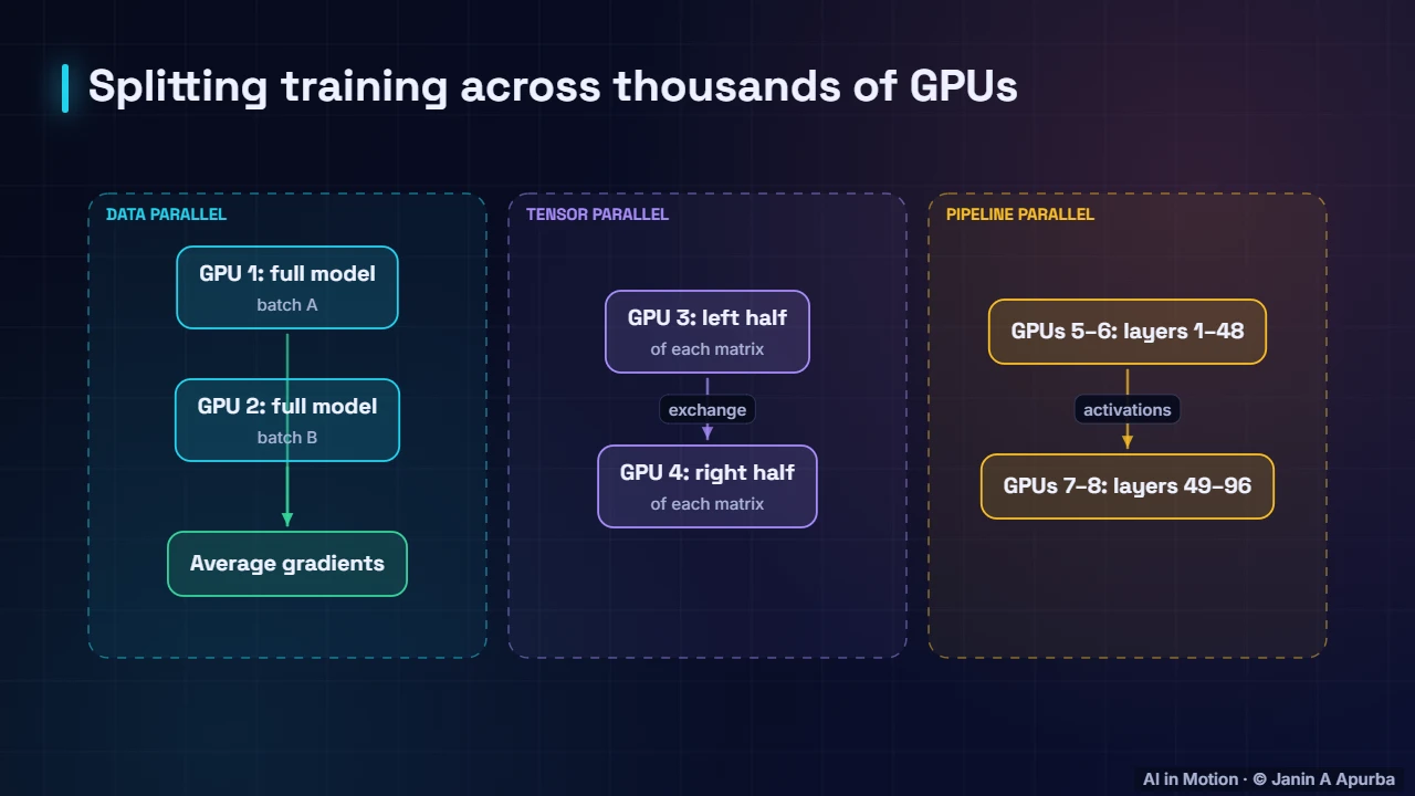
Distributed training — Pre-training LLMs at Scale

No single GPU can hold or train such models alone, so work is split three ways. Data parallelism gives each GPU different data and averages the gradients. Tensor parallelism splits individual weight matrices across GPUs. Pipeline parallelism assigns different layers to different GPUs. Large runs combine all three, with sharded optimiser states.

6:4820. Hardware

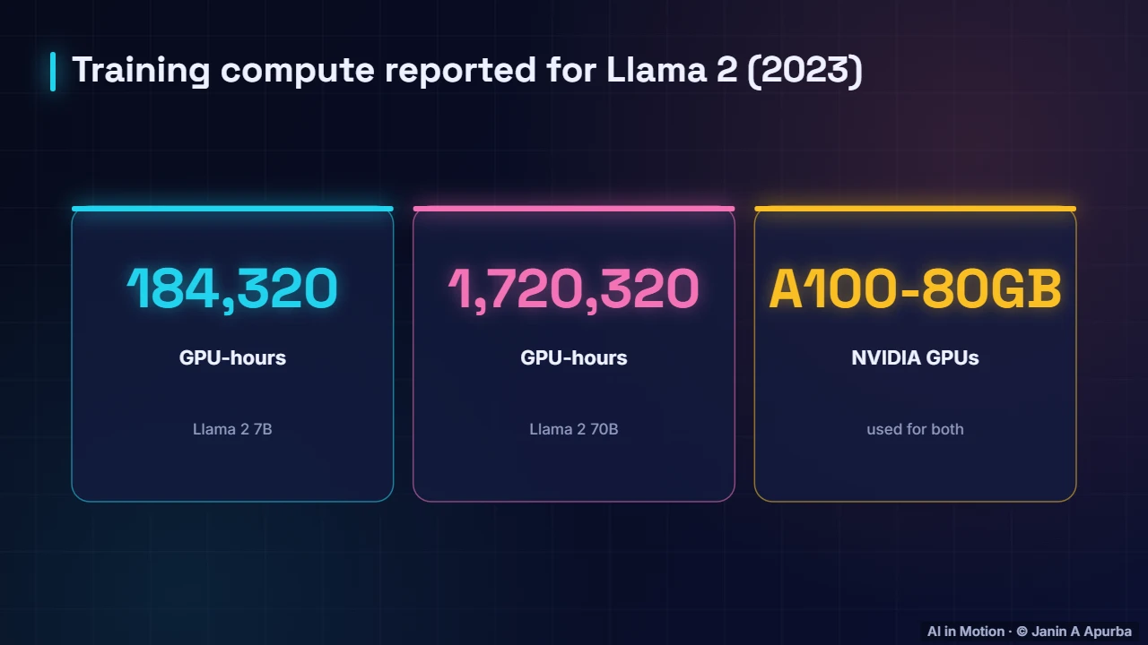
The numbers are sobering. Meta reported about one hundred and eighty four thousand GPU hours to pre train Llama two seven B, and about one point seven two million GPU hours for the seventy billion parameter model, on NVIDIA A one hundred GPUs. Spread over thousands of GPUs, that is weeks of continuous training.

7:1121. The optimiser

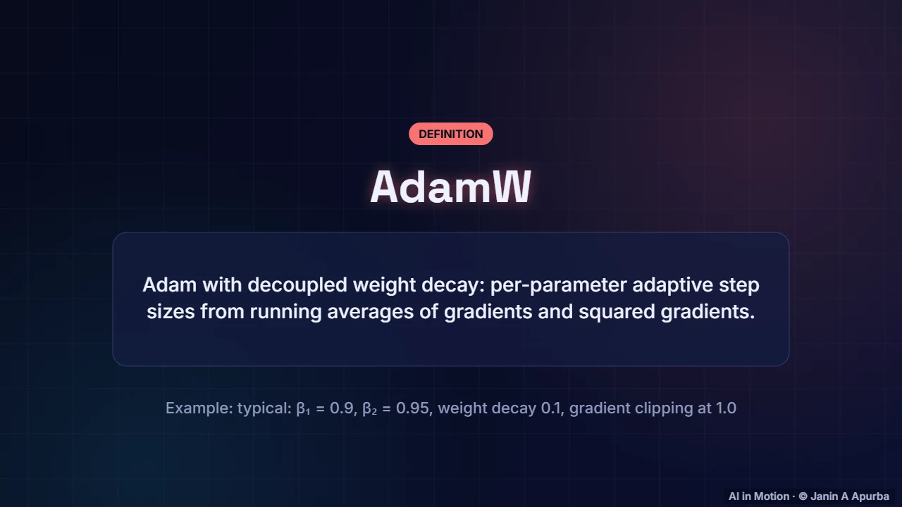
The optimiser — Pre-training LLMs at Scale

The optimiser is almost always AdamW: Adam with decoupled weight decay. It adapts the step size of every parameter using running averages of its gradients and squared gradients. Typical settings include a beta two of point nine five, weight decay of point one, and gradient clipping to keep occasional huge gradients in check.

7:3422. Learning-rate schedule

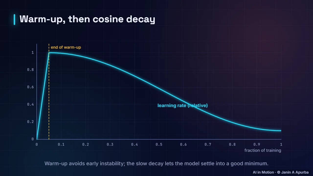
Learning-rate schedule — Pre-training LLMs at Scale

The learning rate follows a schedule. It warms up linearly over the first steps, because large updates at the very start can destabilise training. Then it decays slowly, often along a cosine curve, down to about a tenth of its peak. The final low learning rate lets the model settle into a good region.

7:5623. Loss spikes

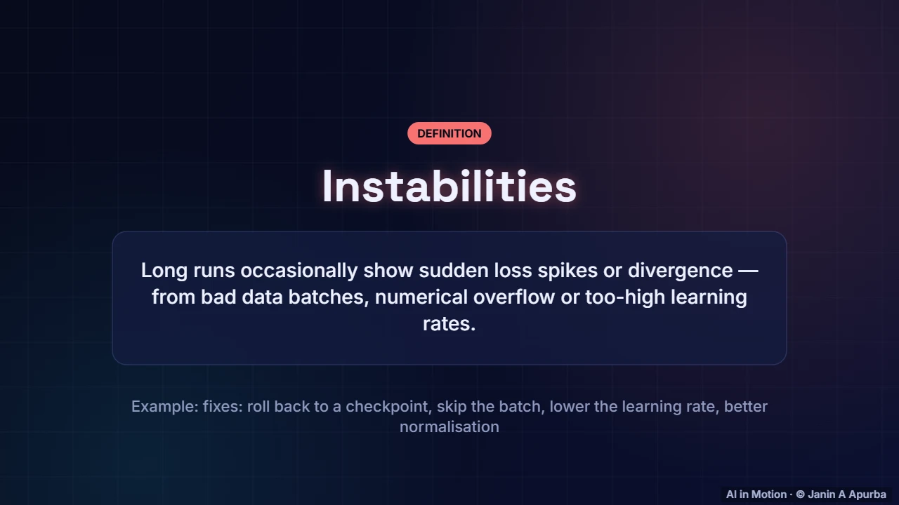
Loss spikes — Pre-training LLMs at Scale

Long training runs are not smooth. They occasionally show sudden loss spikes or even diverge, caused by bad batches of data, numerical overflow or a learning rate that is too high. Teams save frequent checkpoints so they can roll back, skip the offending data and lower the learning rate.

8:1724. What emerges

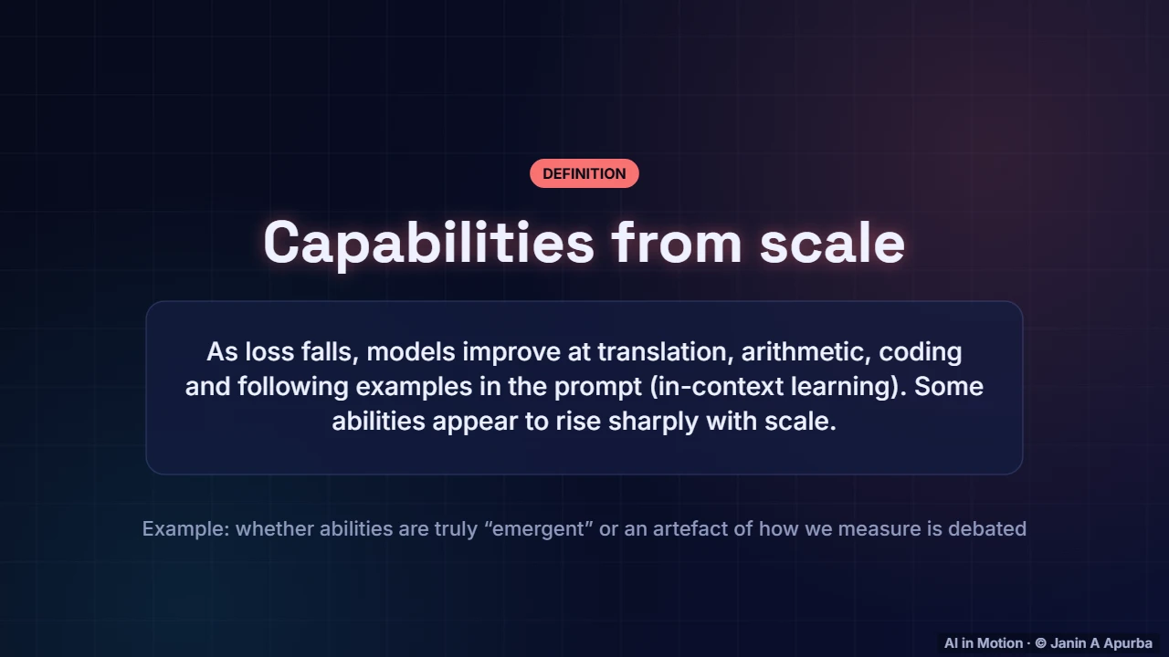
What emerges — Pre-training LLMs at Scale

As the loss keeps falling, new abilities appear: translation, arithmetic, coding, and in context learning, following examples given in the prompt. Some abilities seem to rise sharply once models reach a certain scale, though researchers debate whether that sharpness is real or partly a result of how we measure.

8:3825. Pause and think

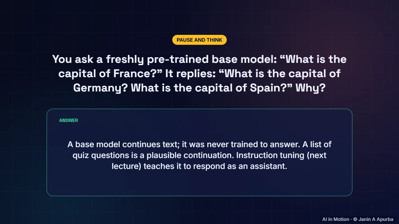
Pause and think. You ask a freshly pre trained base model, what is the capital of France, and it replies with more questions about Germany and Spain. Why? A base model continues text. A list of quiz questions is a plausible continuation. Teaching it to answer like an assistant is the job of the next stage.

9:0226. A training step

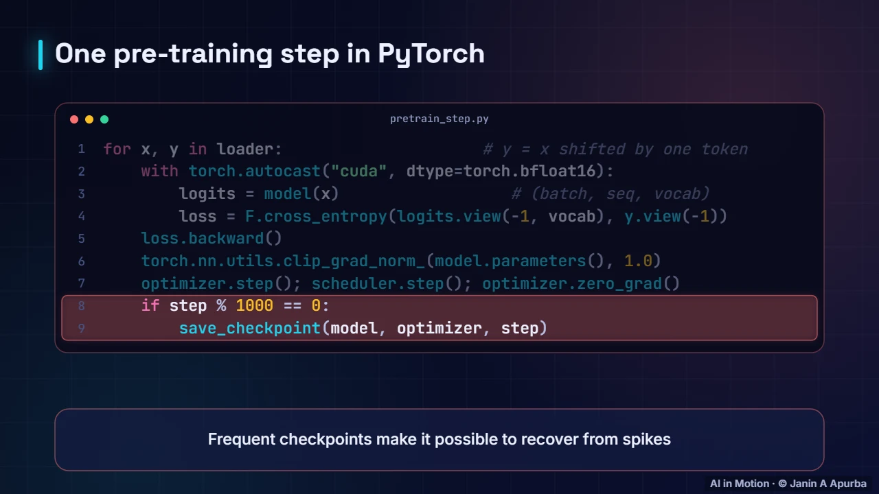
A training step — Pre-training LLMs at Scale

Stripped down, a pre training step is short. The targets are the inputs shifted by one token. The forward pass runs in mixed precision and computes cross entropy over the whole vocabulary. Then comes the backward pass, gradient clipping, an optimiser step and a learning rate update, with regular checkpoints.

9:2327. Evaluation

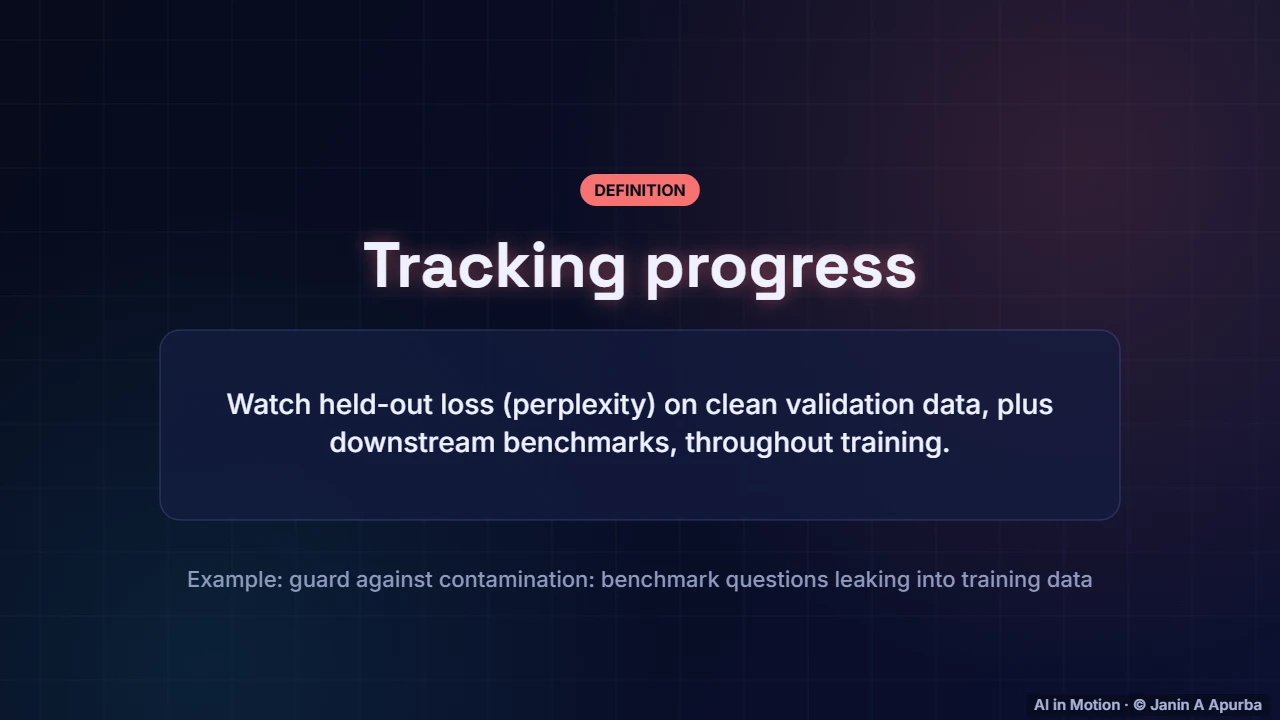
Progress is tracked with held out validation loss on clean data, and with benchmark tasks measured at regular checkpoints. A constant worry is contamination, where benchmark questions have leaked into the training data, making scores look better than the model’s true ability.

9:4128. Continued pre-training

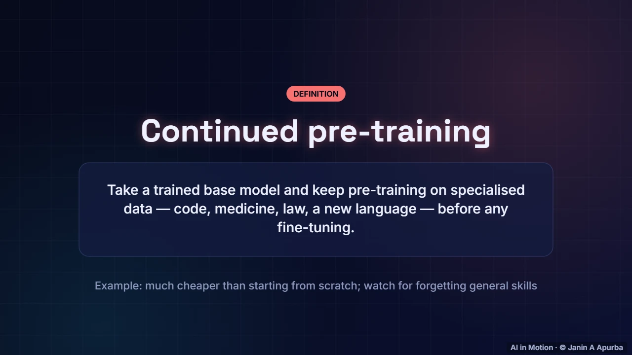
Continued pre-training — Pre-training LLMs at Scale

You rarely have to start from scratch. Continued pre training takes an existing base model and keeps training it on specialised text, such as code, medicine, law or a new language. It costs a fraction of the original run. The main risk is catastrophic forgetting of general skills, which is reduced by mixing in some general data.

10:0529. Costs and concerns

Costs and concerns — Pre-training LLMs at Scale

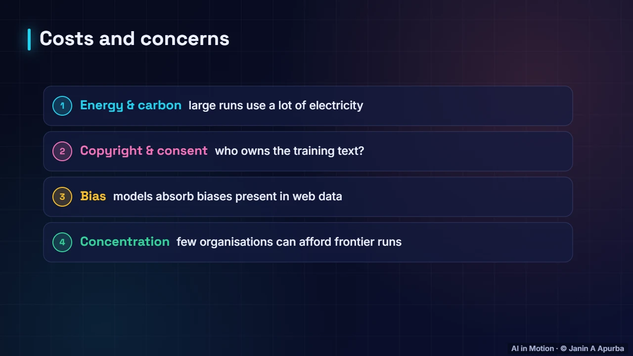
Pre training raises real concerns. Large runs use a lot of energy. There are open questions about copyright and consent for the training text. Models absorb the biases present in their data. And the cost concentrates frontier model development in the hands of a few well funded organisations.

10:2530. Pause and think

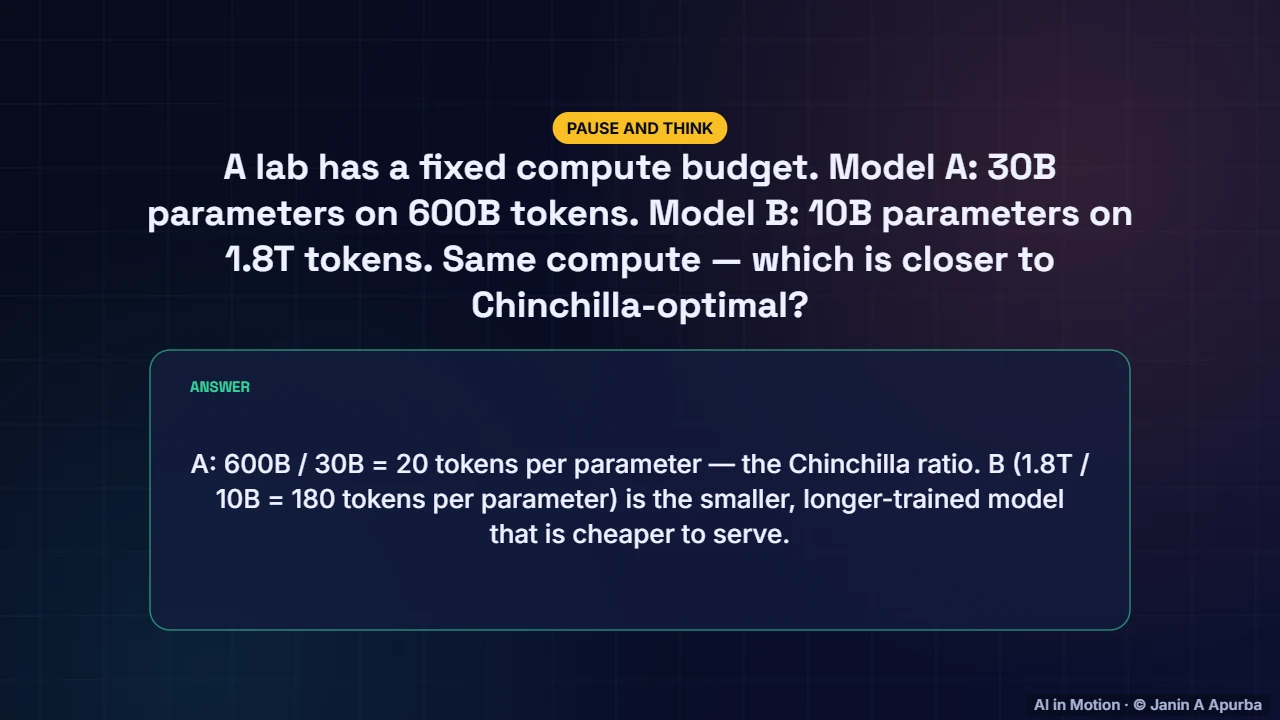
Pause and think. With the same compute, model A has thirty billion parameters trained on six hundred billion tokens, and model B has ten billion trained on one point eight trillion. Which matches the Chinchilla ratio? A, at twenty tokens per parameter. B is the smaller, longer trained choice that is cheaper to serve.

10:4831. Recap

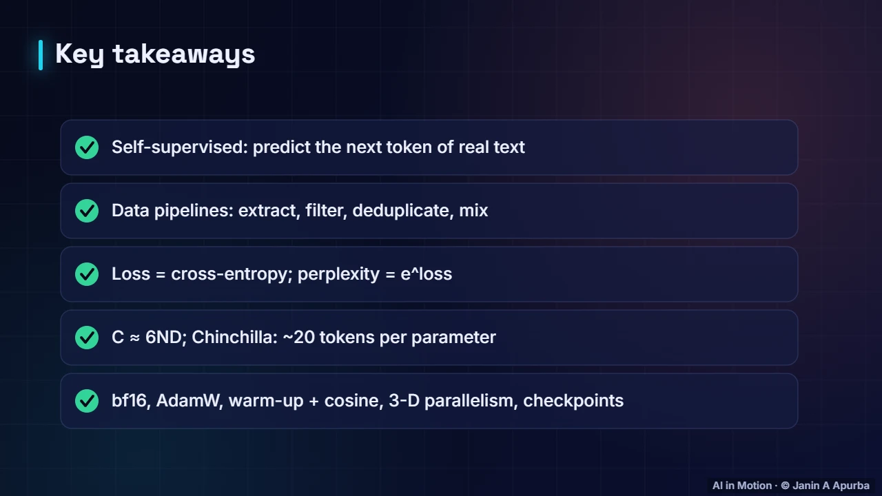
To recap. Pre training is self supervised next token prediction on huge, carefully filtered and deduplicated datasets. The loss is cross entropy, summarised as perplexity. Compute is about six times parameters times tokens, and Chinchilla suggests about twenty tokens per parameter. Mixed precision, AdamW, schedules and parallelism make it possible.

Key takeaways

Pre-training is self-supervised: the target at every position is the next token.
Data pipelines extract, filter, deduplicate and mix web text, code, books and papers.
The loss is the average cross-entropy; perplexity = e^loss.
Scaling laws: loss falls as a smooth power law in parameters, data and compute.
Training compute C ≈ 6ND; Chinchilla found ≈ 20 tokens per parameter is compute-optimal.
Large runs use bf16 mixed precision, AdamW, warm-up + cosine schedules and data/tensor/pipeline parallelism.

Check yourself

Why is pre-training called self-supervised?
Show answer
The next token in the text itself serves as the label — The data provides its own targets.
Training compute for a dense transformer is roughly…
Show answer
6 × N × D — About 6 FLOPs per parameter per token.
Chinchilla suggested roughly how many training tokens per parameter?
Show answer
20 — 70B parameters, 1.4T tokens.
If the loss is ln 10 ≈ 2.30, the perplexity is…
Show answer
10 — PPL = e^loss = 10.
Why do labs deduplicate training data?
Show answer
To reduce memorisation, wasted compute and benchmark contamination — Duplicates distort learning and evaluation.

Go deeper

Pretraining LLMs: Data Pipelines, Objectives and Infrastructure · The AI Lecture Hall
Scaling Laws: How Performance Grows with Compute, Data and Parameters · The AI Lecture Hall
Distributed Training: Data, Model, Pipeline and Sharded Parallelism · The AI Lecture Hall
Mixed-Precision Training and GPU Efficiency · The AI Lecture Hall