Inside a Large Language Model — lecture notes
Follow a sentence through a GPT-style model: tokens, embeddings, the residual stream, attention and MLP blocks, layer norms, unembedding and sampling — with real parameter counts.
0:001. Introduction
Large language models can write essays, code and poems, but underneath they perform one surprisingly simple task, over and over. In this deep dive we open the box and follow a sentence through a GPT style model, layer by layer, until the next word pops out.
0:192. Scale
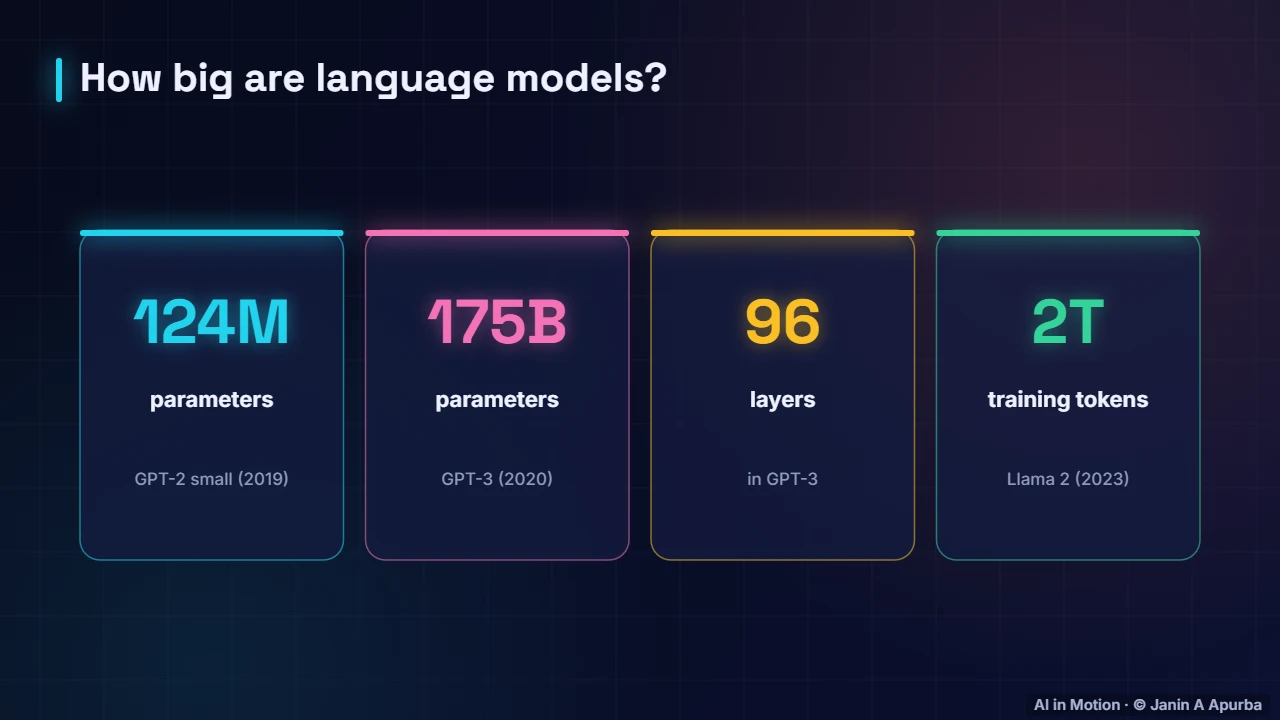
Language models come in many sizes. The smallest GPT two had one hundred and twenty four million parameters. GPT three had one hundred and seventy five billion, stacked in ninety six layers. Llama two was trained on two trillion tokens of text. Yet the same architecture runs at every scale.
0:403. What is a language model?
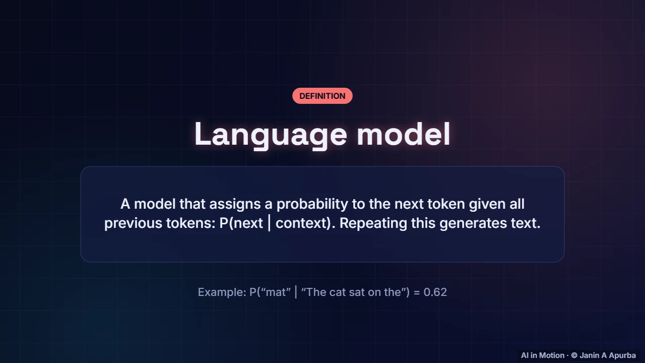
A language model is a machine that predicts the next token. Given all the text so far, it outputs a probability for every possible next token in its vocabulary. Choose one, append it, and ask again. Every chatbot answer is produced by repeating this single step, one token at a time.
1:024. Generating text
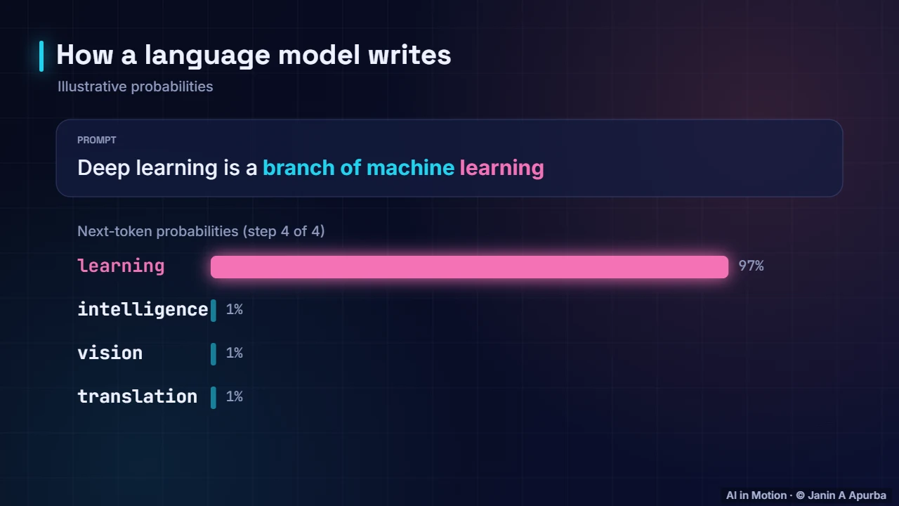
Here is the loop in action. The model reads the prompt, produces a probability distribution over candidates, picks one, appends it, and repeats. Nothing is planned in advance at the level of whole sentences, yet coherent paragraphs emerge because every prediction is conditioned on everything written so far.
1:225. The big picture
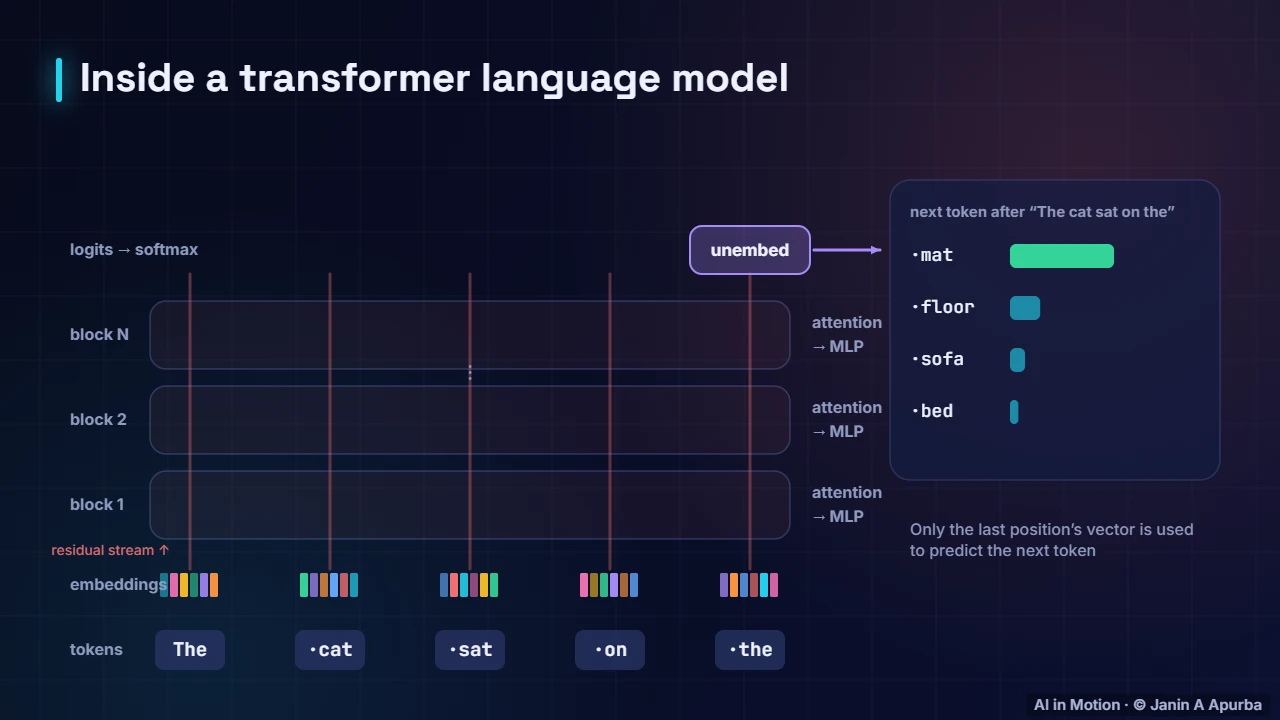
This is the whole journey in one picture. Tokens become embedding vectors. The vectors flow up through a stack of identical transformer blocks, each containing an attention step and an MLP step. At the top, the last position’s vector is turned into scores for every token in the vocabulary.
1:436. Step 1: tokens
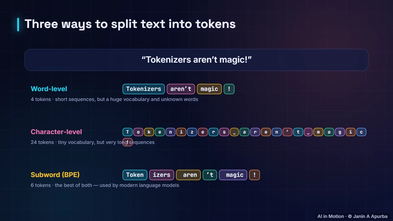
The first step is tokenisation. Text is split into tokens, which are usually pieces of words. Common words are single tokens, while rare words are broken into several pieces. A typical English word is about one point three tokens, and models see tokens, never raw letters.
2:037. Building the vocabulary
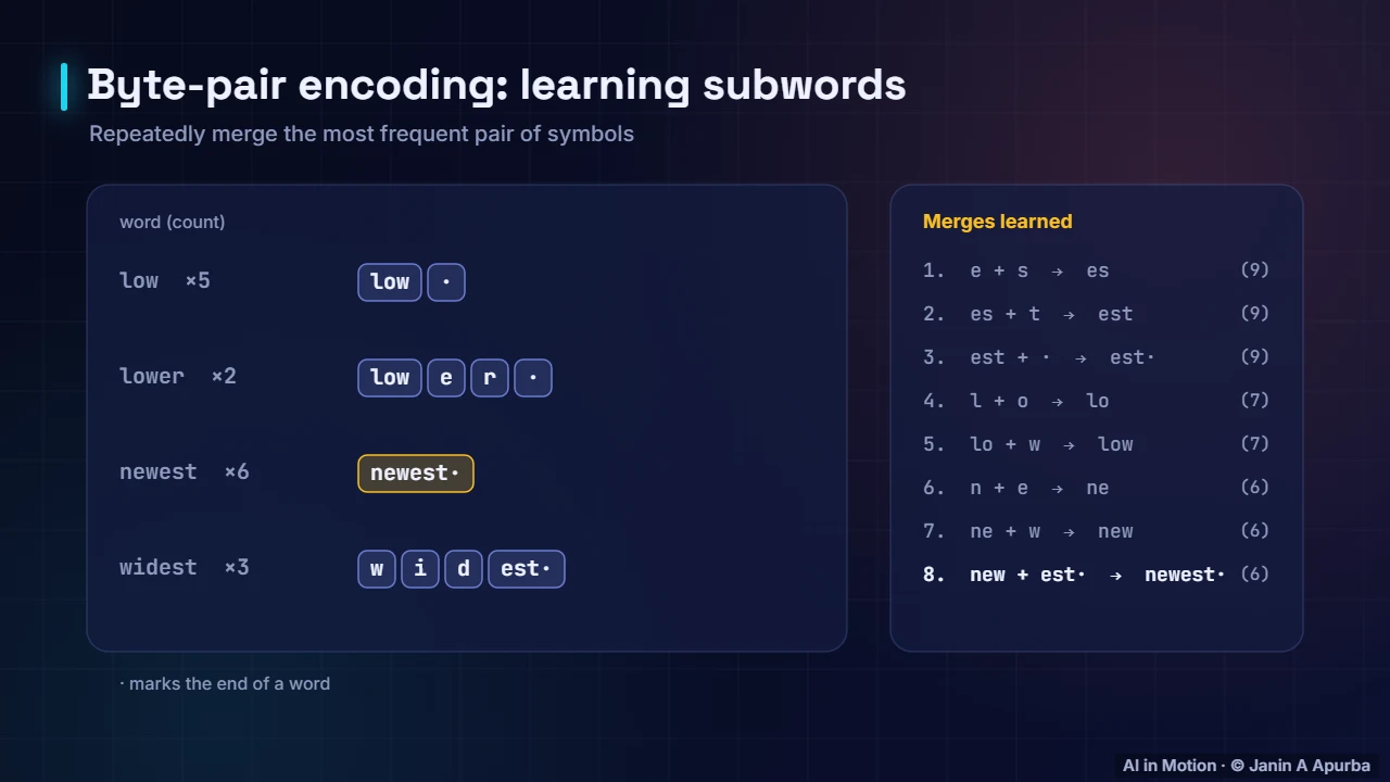
The vocabulary is usually built with byte pair encoding. Start from single characters, then repeatedly merge the most frequent adjacent pair into a new token. After tens of thousands of merges you have a vocabulary where frequent words and pieces get their own tokens. GPT two used about fifty thousand.
2:248. Step 2: embeddings
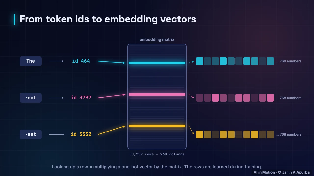
Each token id selects one row of the embedding matrix, turning the token into a vector of numbers. In GPT two small, each vector has seven hundred and sixty eight numbers. These rows are learned during training, so tokens used in similar ways end up with similar vectors.
2:449. Pause and think
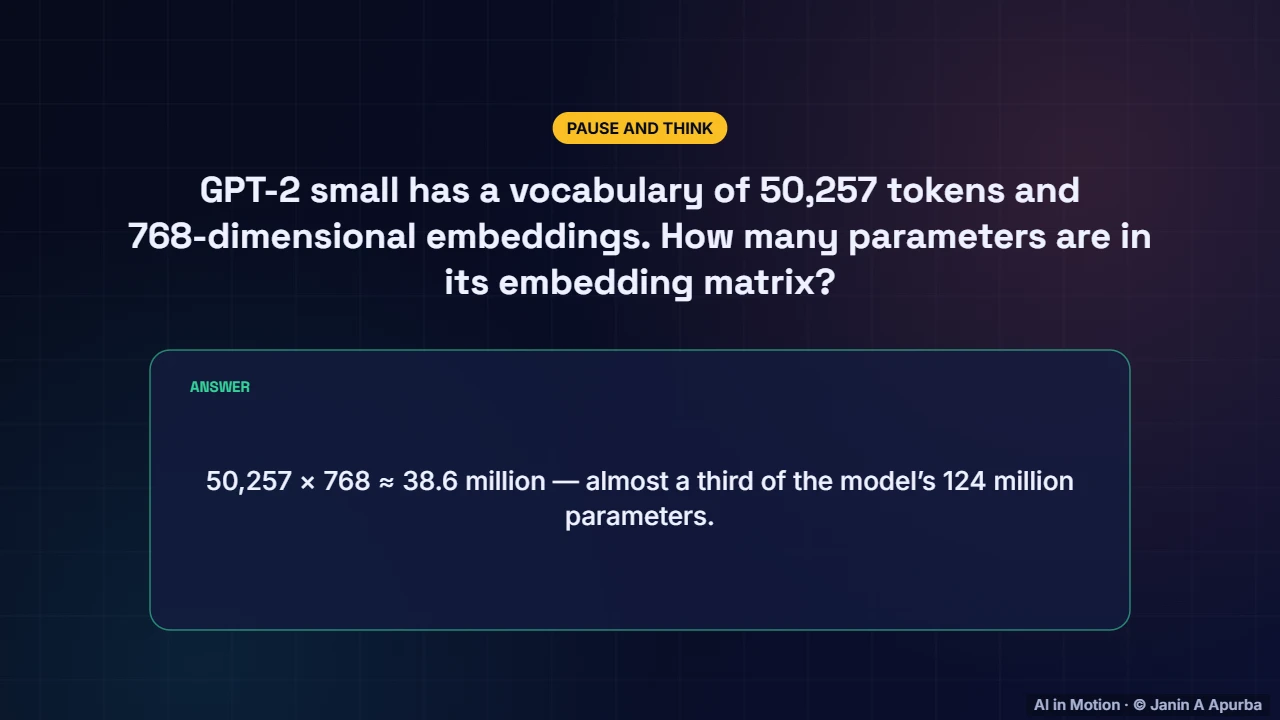
Pause and think. GPT two small has a vocabulary of fifty thousand, two hundred and fifty seven tokens, with seven hundred and sixty eight dimensional embeddings. How many parameters does the embedding matrix hold? About thirty eight point six million, almost a third of the whole model.
3:0410. Where is each token?
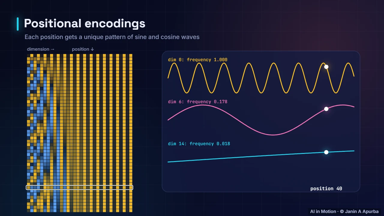
Embeddings alone ignore word order: dog bites man and man bites dog would look identical. So position information is added. The original transformer added sinusoidal patterns like these, each dimension waving at a different frequency. Modern models usually rotate queries and keys instead, a method called RoPE.
3:2511. The residual stream
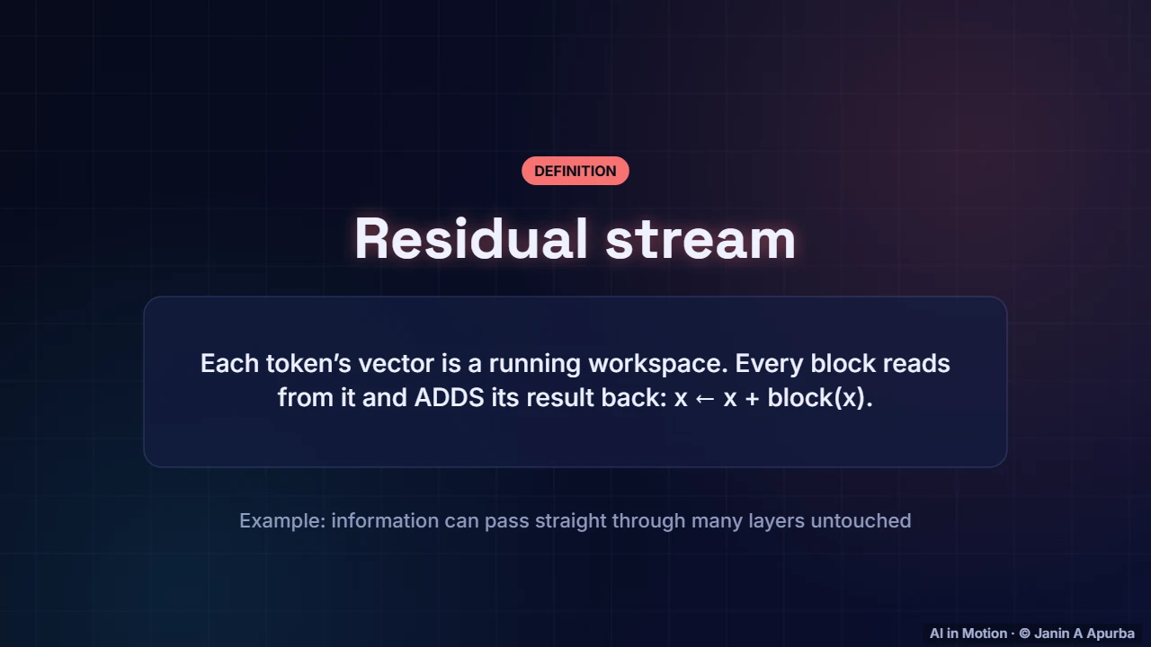
Think of each token’s vector as a running workspace called the residual stream. Every block reads from the stream, computes something, and adds its result back. Because blocks add rather than overwrite, information can flow straight through dozens of layers, and gradients flow back just as easily during training.
3:4512. One transformer block
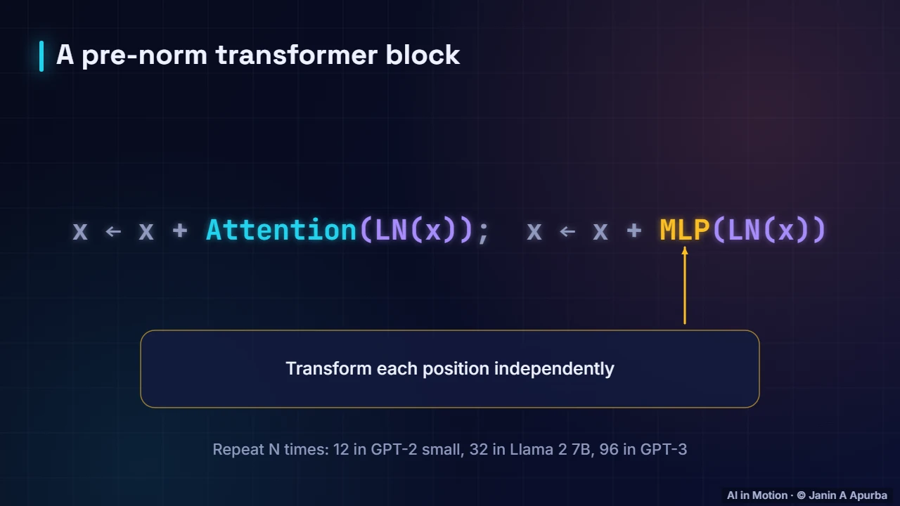
Each block does two things. First, attention mixes information between positions. Second, a small feed forward network, the MLP, transforms each position on its own. Both read a normalised copy of the stream and add their output back. Stack twelve, thirty two or ninety six of these blocks, and you have a model.
4:0813. Attention moves information
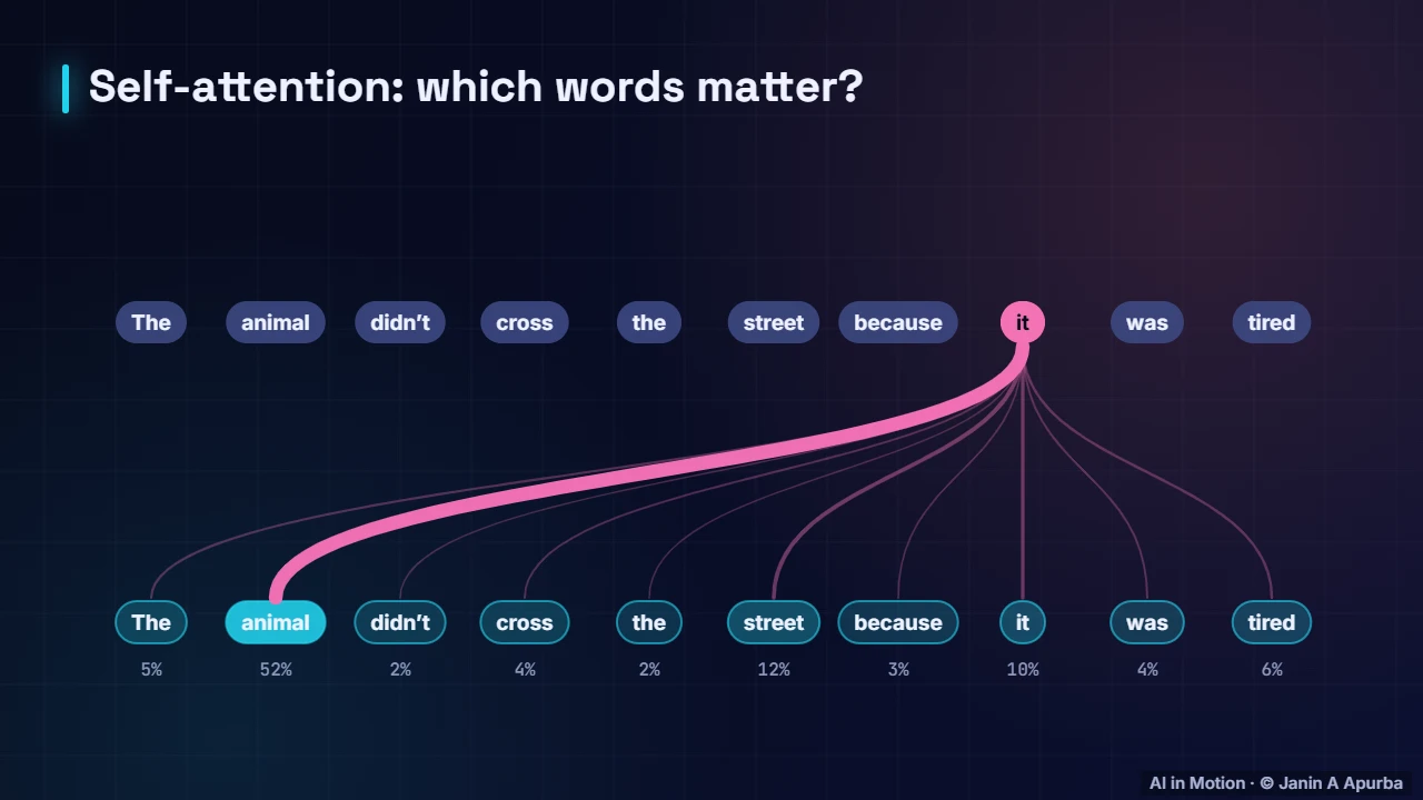
Attention is how tokens share information. Each position asks a question, compares it with every earlier position, and gathers information from the most relevant ones. Here the word it looks back and gathers meaning from the noun it refers to. The next lecture covers the mathematics in detail.
4:2814. No peeking ahead
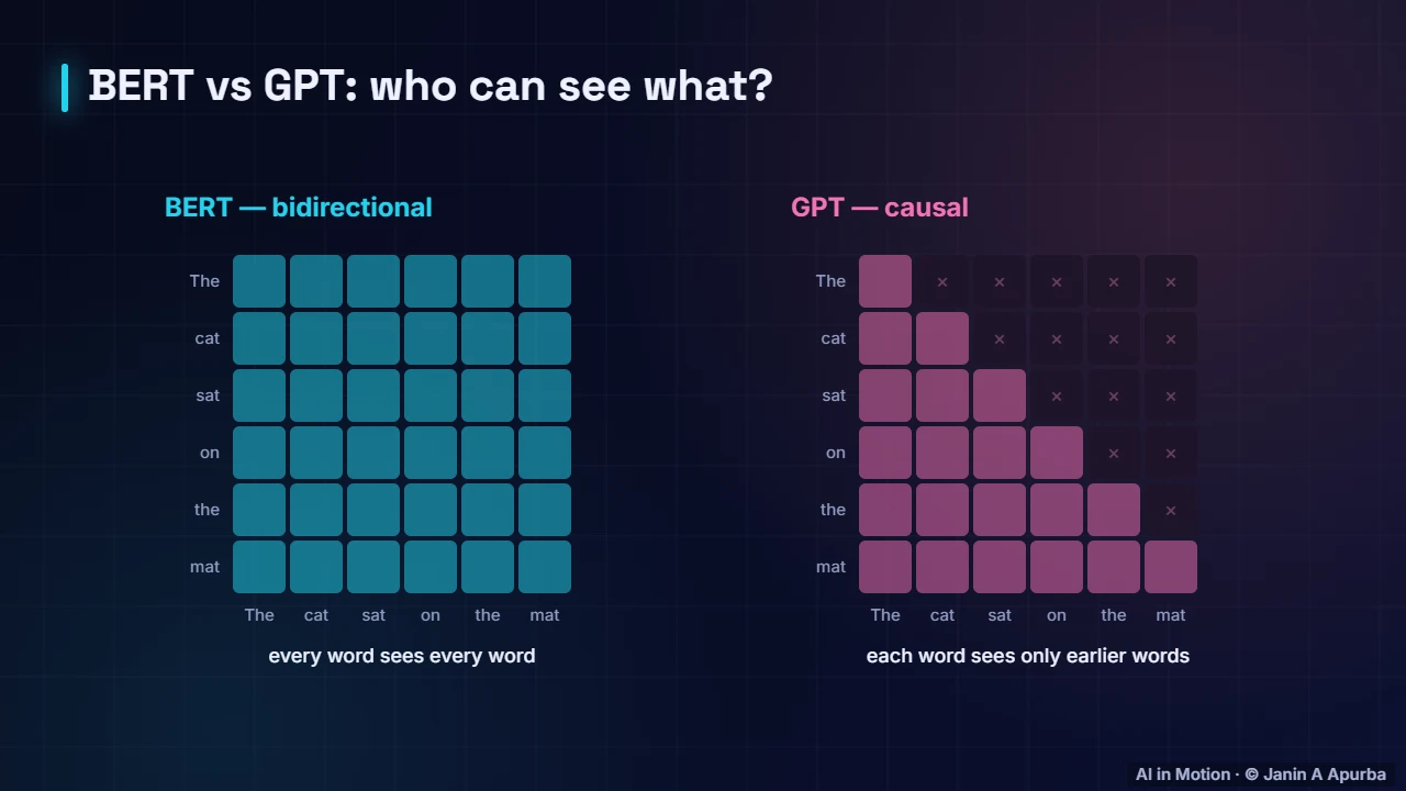
A GPT style model uses a causal mask: each position may only attend to itself and earlier positions, never to the future. That is what makes it a next token predictor. BERT, in contrast, sees the whole sentence in both directions, which suits understanding tasks but not free generation.
4:4915. The MLP layer
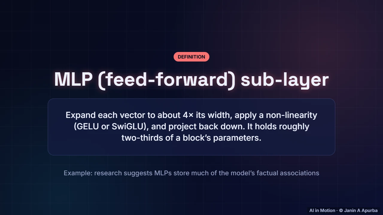
The MLP sub layer processes each position on its own. It expands the vector to about four times its width, applies a non linear activation, and projects it back down. It holds about two thirds of each block’s parameters, and research suggests it stores much of the model’s factual knowledge.
5:1016. GELU
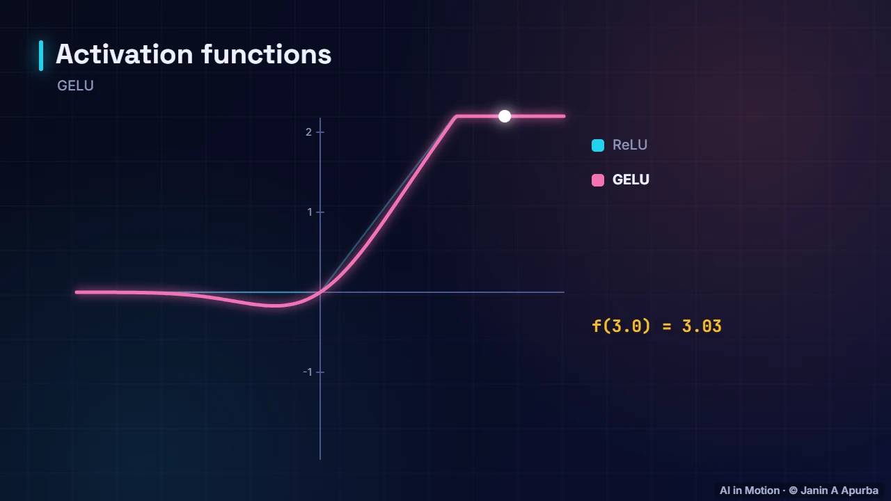
GPT models use the GELU activation, a smooth cousin of ReLU that lets a little negative signal through near zero. Newer models such as Llama use a gated variant called SwiGLU. These small non linear bends between the big matrix multiplications are what let the network represent complicated functions.
5:3117. Layer normalisation
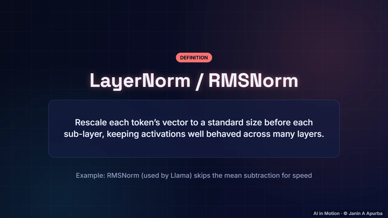
Before each sub layer, the vector is normalised to a standard size. This layer normalisation keeps the numbers in a healthy range as they pass through dozens of blocks, making deep stacks trainable. Llama uses a slightly cheaper variant called RMS norm.
5:4918. Many heads
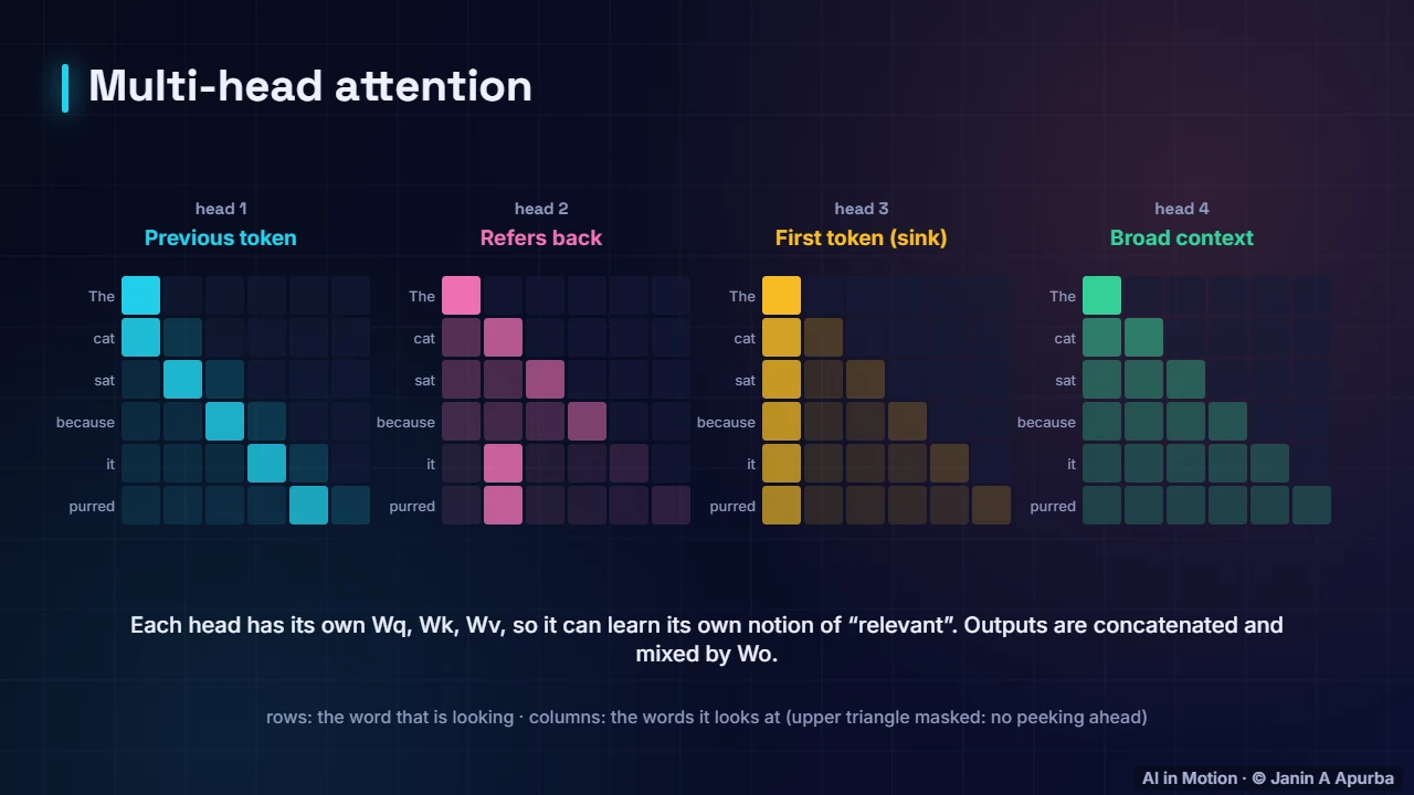
Attention is split into several heads that work in parallel, each with its own projections. Different heads learn different jobs: one tracks the previous token, one links pronouns to nouns, one attends broadly. GPT two small has twelve heads per layer, and GPT three has ninety six.
6:0919. Unembedding
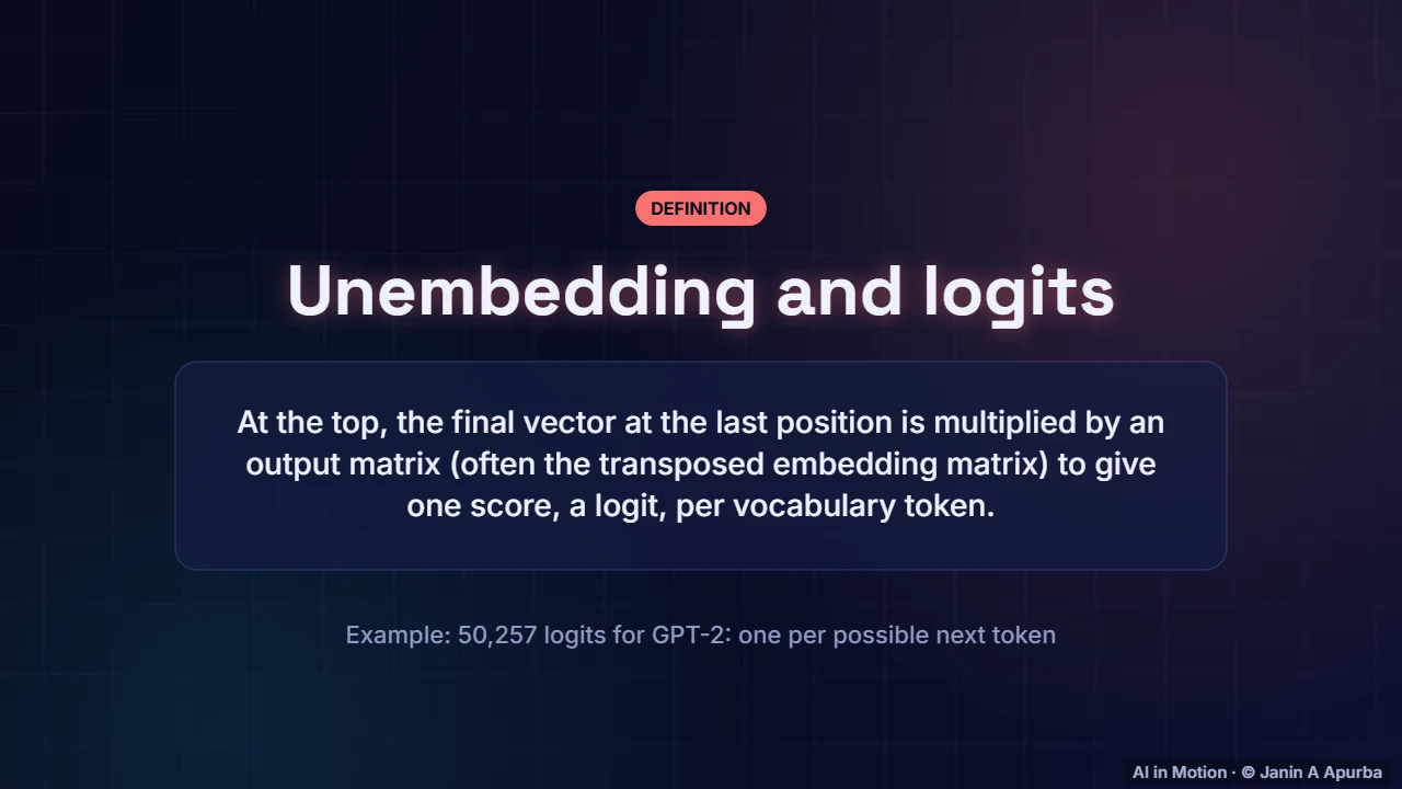
At the top of the stack, the vector at the last position is multiplied by an output matrix, often the transpose of the embedding matrix, a trick called weight tying. The result is one score, called a logit, for every token in the vocabulary: fifty thousand scores for GPT two.
6:3020. From logits to a choice
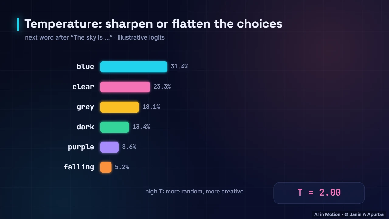
The softmax function turns logits into probabilities. Then we choose. Always picking the most likely token is deterministic but can be dull and repetitive. Sampling with a temperature adds variety: low temperature sharpens the distribution, high temperature flattens it and makes the model more adventurous.
6:5021. Pause and think
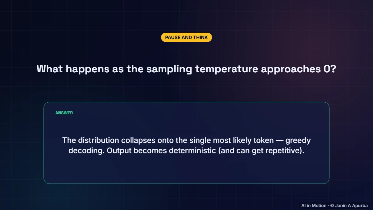
Pause and think. What happens as the temperature approaches zero? The softmax becomes infinitely sharp, all probability collapses onto the single most likely token, and sampling turns into greedy decoding. The output becomes deterministic, which is useful for code or facts but can become repetitive for creative text.
7:1022. Parameter budget
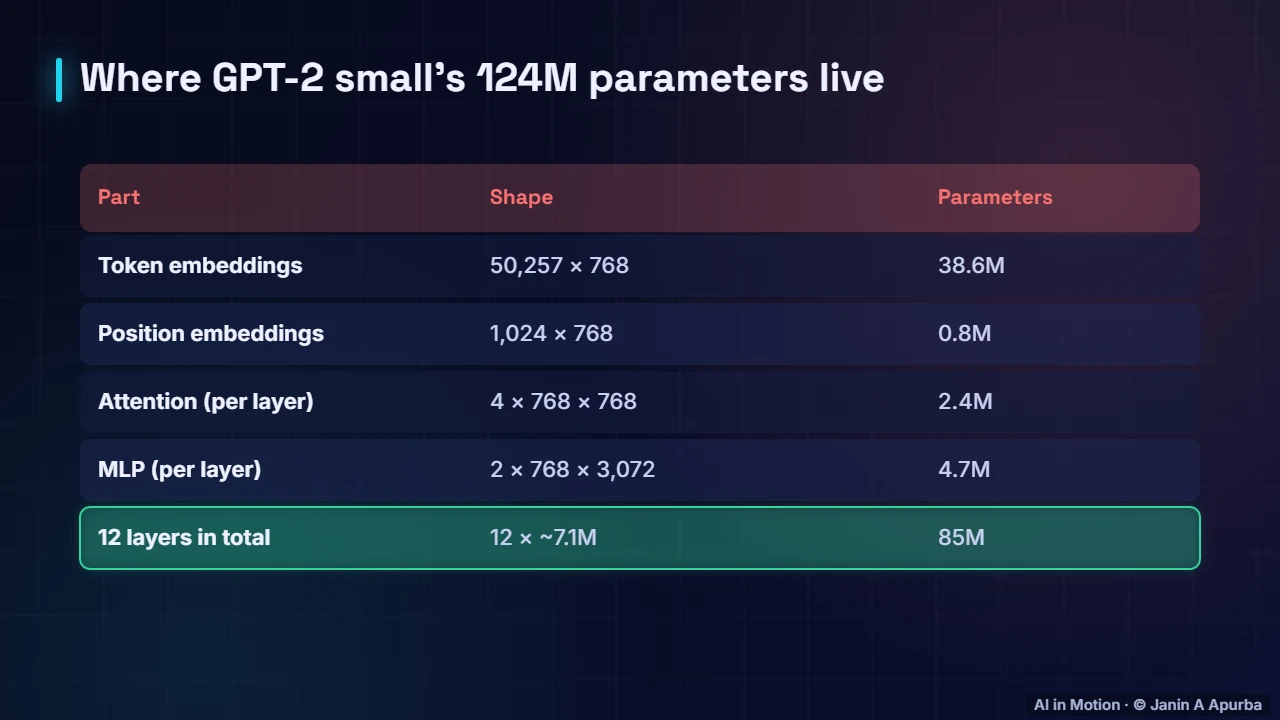
Where do the parameters live? In GPT two small, token embeddings take thirty eight point six million. Each layer’s attention holds about two point four million, and each MLP about four point seven million. Twelve layers make about eighty five million, and together the total is one hundred and twenty four million.
7:3223. The context window
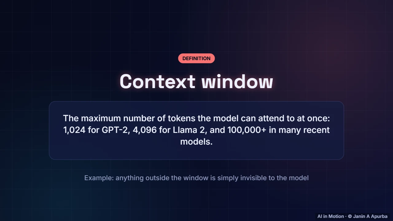
Every model has a context window, the maximum number of tokens it can look at in one go. GPT two could see one thousand and twenty four tokens, Llama two four thousand, and many recent models over a hundred thousand. Anything outside the window is simply invisible.
7:5224. Sliding out of view
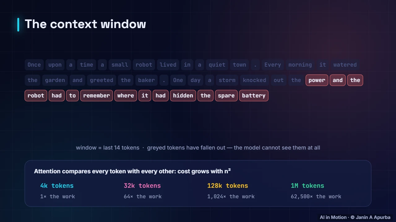
Here the window holds the last fourteen tokens. As new text streams in, older tokens fall out and the model can no longer see them at all. Longer windows help, but attention compares every token with every other, so doubling the context roughly quadruples the attention work.
8:1225. The generation loop
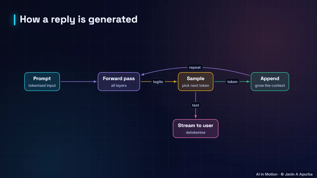
Putting it together, a reply is generated in a loop. The prompt is tokenised and passed through every layer, producing logits. One token is sampled and appended to the context, then the loop runs again. Each token is streamed to the user as it arrives, which is why answers appear word by word.
8:3426. A popular variant
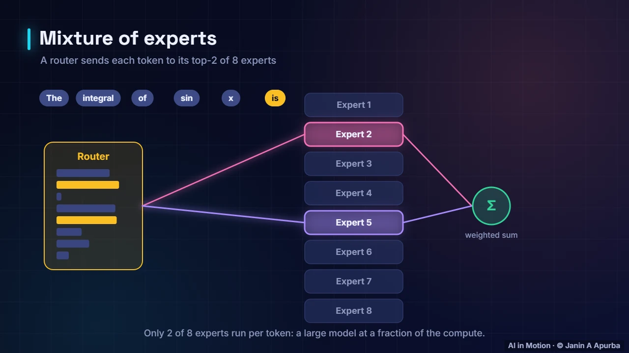
A popular variant is the mixture of experts. The MLP in each block is replaced by several expert MLPs, and a small router sends each token to only a couple of them. The model can hold many more parameters while each token uses only a fraction, keeping computation per token modest.
8:5627. Decoder vs encoder
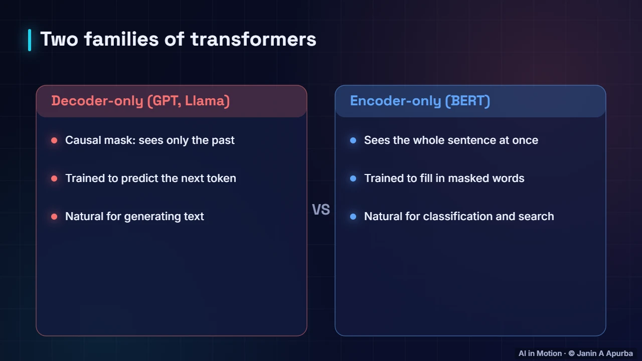
Transformers come in two main families. Decoder only models, like GPT and Llama, use a causal mask and predict the next token, which makes them natural generators. Encoder only models, like BERT, see the whole sentence and fill in blanks, which suits classification and search. Encoder decoder models such as T5 combine both.
9:1828. Running a model
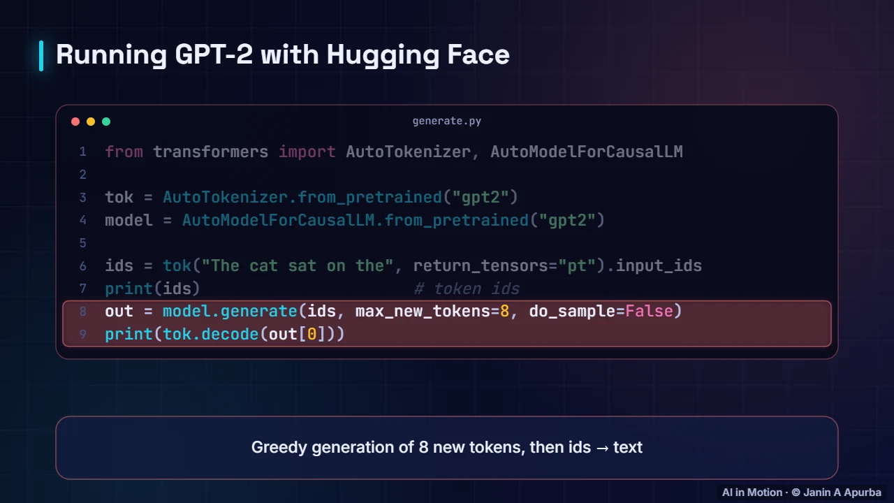
You can run this whole pipeline on a laptop. With the Hugging Face transformers library, load the GPT two tokenizer and model, turn text into token ids, and call generate. Setting do sample to false gives greedy decoding. The output ids are decoded back into text.
9:3829. Pause and think
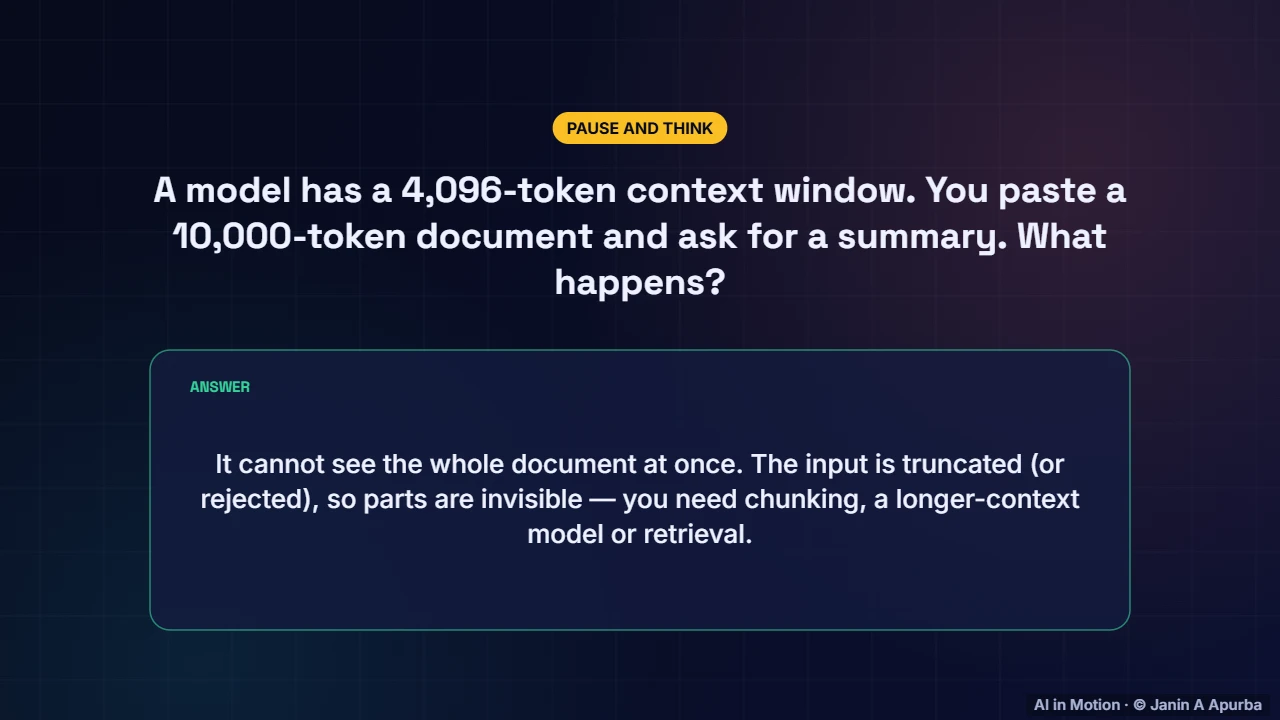
Pause and think. A model has a four thousand token context window, and you paste in a ten thousand token document for a summary. What happens? It simply cannot see the whole document. The input is truncated or rejected, so you need chunking, a longer context model, or retrieval.
9:5930. Limitations
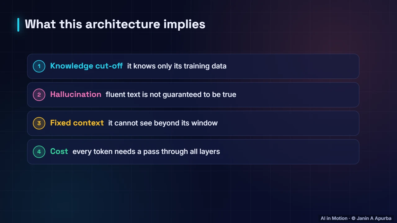
This architecture has consequences. The model knows only what was in its training data, up to a cut off date. It produces fluent text that is not guaranteed to be true, which we call hallucination. It cannot see beyond its window, and every single token requires a pass through all the layers.
10:2131. Recap
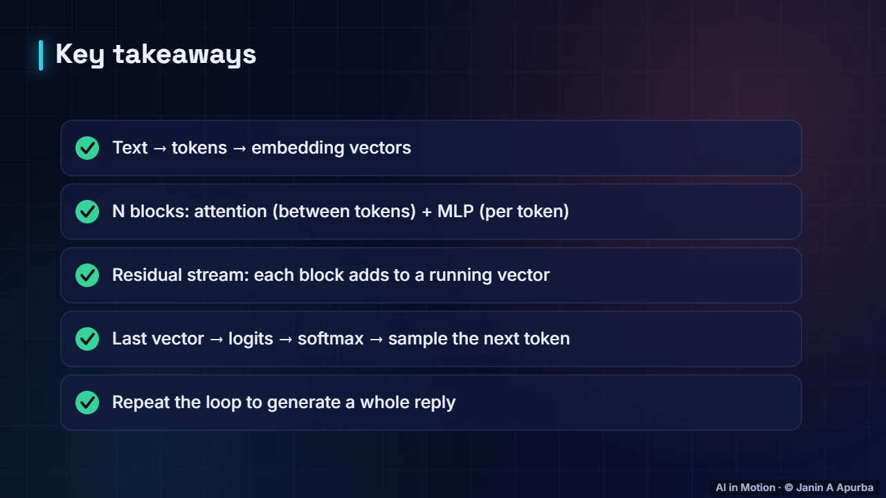
To recap. Text becomes tokens and then embedding vectors. The vectors flow through a stack of blocks, where attention mixes information between tokens and the MLP transforms each one, all adding to a residual stream. The last vector becomes logits, a token is sampled, and the loop repeats.
Key takeaways
- A language model predicts a probability distribution over the next token; generation repeats this step.
- Text is split into subword tokens (BPE) and each token id selects an embedding vector.
- Transformer blocks add attention (mixing between positions) and MLP (per-position) outputs to a residual stream.
- A causal mask lets each position see only earlier tokens.
- The final vector is unembedded into logits; softmax and sampling (temperature) choose the next token.
- GPT-2 small: 124M parameters, 12 layers, 768 dimensions, 50,257-token vocabulary.
Check yourself
- What does a decoder-only language model predict at each step?
Show answer
A probability distribution over the next token — Generation repeats next-token prediction.
- What is the residual stream?
Show answer
The running vector each block reads from and adds its output to — Blocks add, rather than overwrite.
- Why do GPT-style models use a causal mask?
Show answer
So each position can only attend to earlier positions, enabling next-token prediction — The model must not see the future it is predicting.
- Setting temperature close to 0 makes sampling…
Show answer
Nearly greedy and deterministic — Probability concentrates on the top token.
- Roughly how many parameters does GPT-2 small have?
Show answer
124 million — 124M, of which 38.6M are token embeddings.
Go deeper
- Large Language Models: What They Are and How They Are Built · The AI Lecture Hall
- The Transformer Architecture Explained, Block by Block · The AI Lecture Hall
- The GPT Family: Autoregressive Language Models from GPT-1 to Today · The AI Lecture Hall
© 2026 Janin A Apurba, CSE, AUST · Advanced ICT Officer, CNRS-UNHCR. All rights reserved. Notes for the animated lecture at https://ai-in-motion.vercel.app/watch/inside-a-large-language-model.html