GANs and VAEs: A Deep Dive into Generative Models — lecture notes
Two classic ways to generate data: autoencoders and variational autoencoders (ELBO, KL, reparameterisation), and generative adversarial networks (the minimax game, mode collapse, DCGAN, WGAN, conditional and cycle GANs, StyleGAN) — with evaluation and a comparison with diffusion.
0:001. Introduction
Before diffusion models took over, two families dominated generative AI: variational autoencoders and generative adversarial networks. They are still widely used, and they contain ideas that every modern generator builds on. In this deep dive we take both apart and compare them.
0:182. Learning the data itself
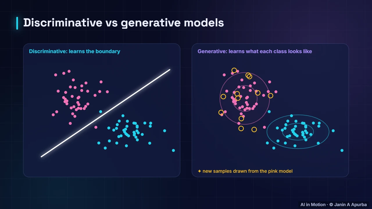
A generative model learns the distribution of the data itself, not just a boundary between classes. Once it knows the shape of the data, it can draw brand new samples from it, the amber circles. Both VAEs and GANs learn to turn simple random noise into samples that look like real data.
0:403. Latent variables
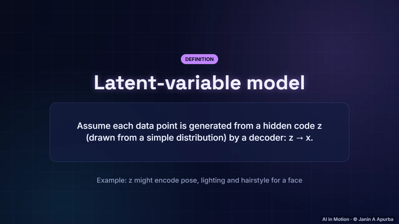
Both families are latent variable models. They imagine that each data point was generated from a hidden code, z, drawn from a simple distribution such as a standard normal, and passed through a decoder network. For faces, dimensions of z might come to control pose, lighting or hairstyle.
1:004. Autoencoders
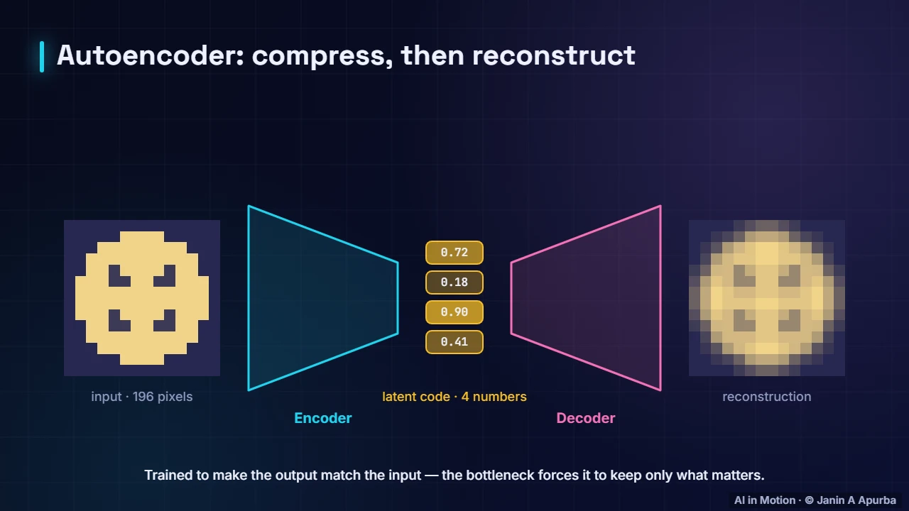
Start with a plain autoencoder. The encoder squeezes a one hundred and ninety six pixel image into a code of just four numbers, and the decoder tries to rebuild the image from those four numbers. Training minimises the difference, so the bottleneck is forced to keep only the essential information.
1:215. Denoising autoencoders
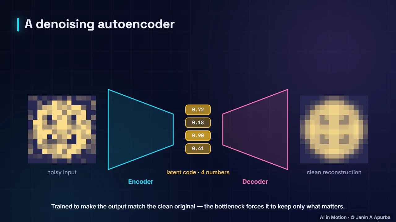
A denoising autoencoder is given a noisy version of the image but trained to output the clean original. To succeed, it must learn what real images look like, so it can remove noise it has never seen before. This denoising idea returns, in a much bigger form, in diffusion models.
1:426. Why plain autoencoders cannot generate
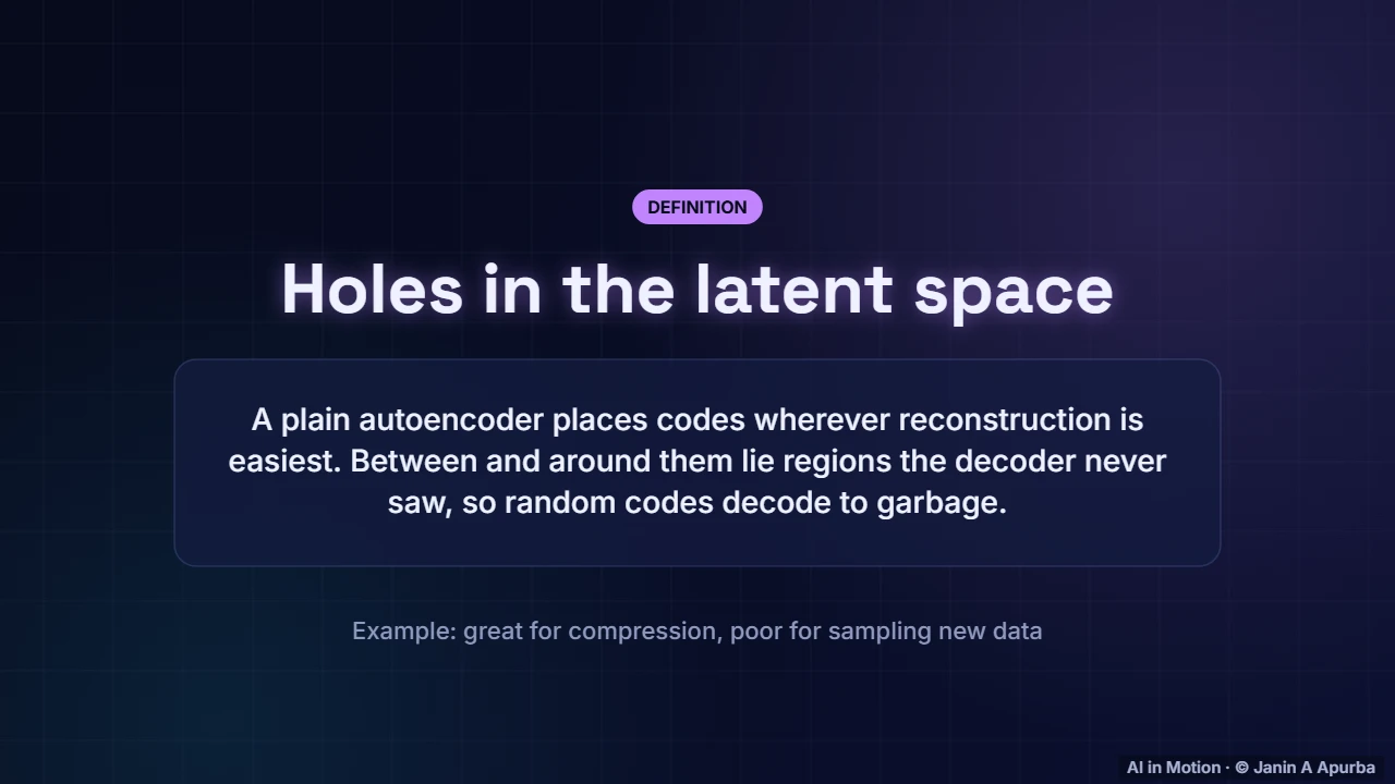
Can we generate new images by feeding random codes to the decoder? Not reliably. A plain autoencoder places codes wherever reconstruction is easiest, leaving holes between them. A random code usually lands in a hole the decoder never saw, and decodes to garbage. We need a better organised latent space.
2:047. Variational autoencoders
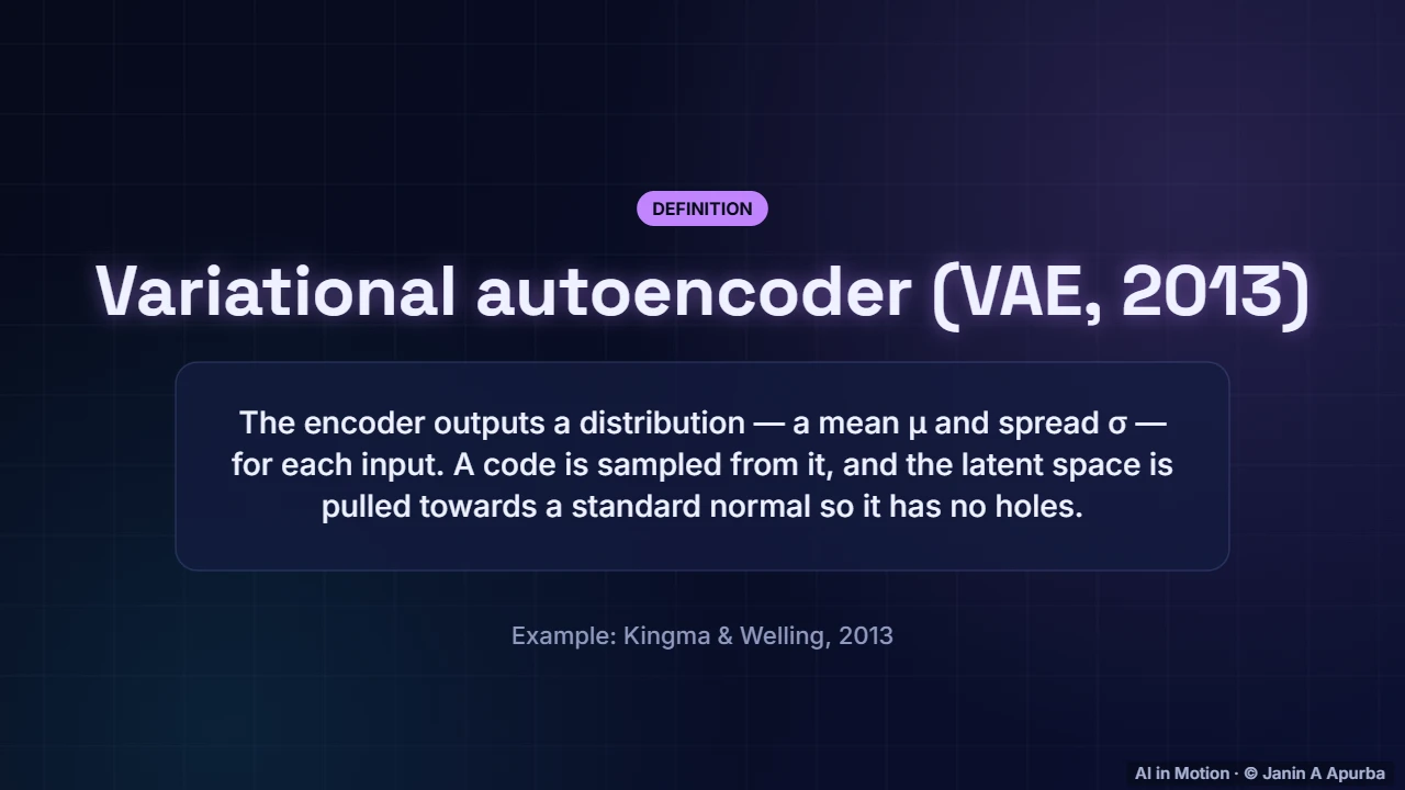
The variational autoencoder, introduced by Kingma and Welling in 2013, fixes this. Its encoder outputs a small probability cloud for each input, a mean and a spread, instead of a single point. A code is sampled from the cloud, and a penalty pulls all the clouds towards a standard normal distribution, filling in the holes.
2:278. The VAE objective
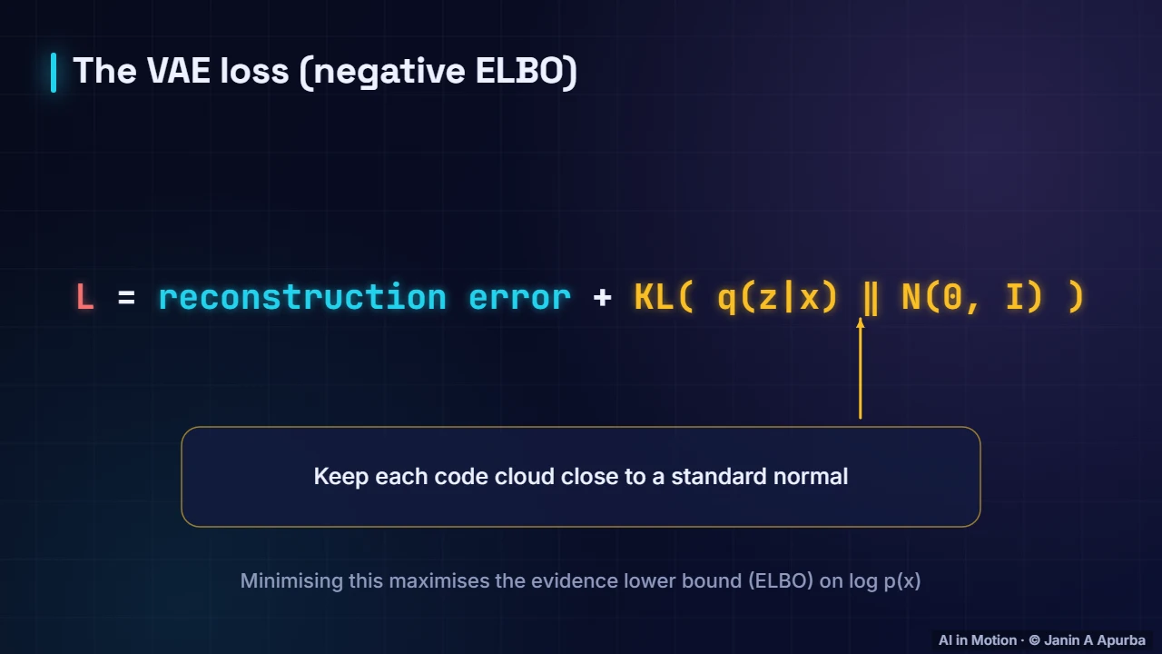
The VAE loss has two terms. The reconstruction term asks the decoder to rebuild the input from a sampled code. The KL term keeps each code cloud close to a standard normal. Together they maximise a lower bound on the likelihood of the data, called the evidence lower bound, or ELBO.
2:489. Pulling codes together
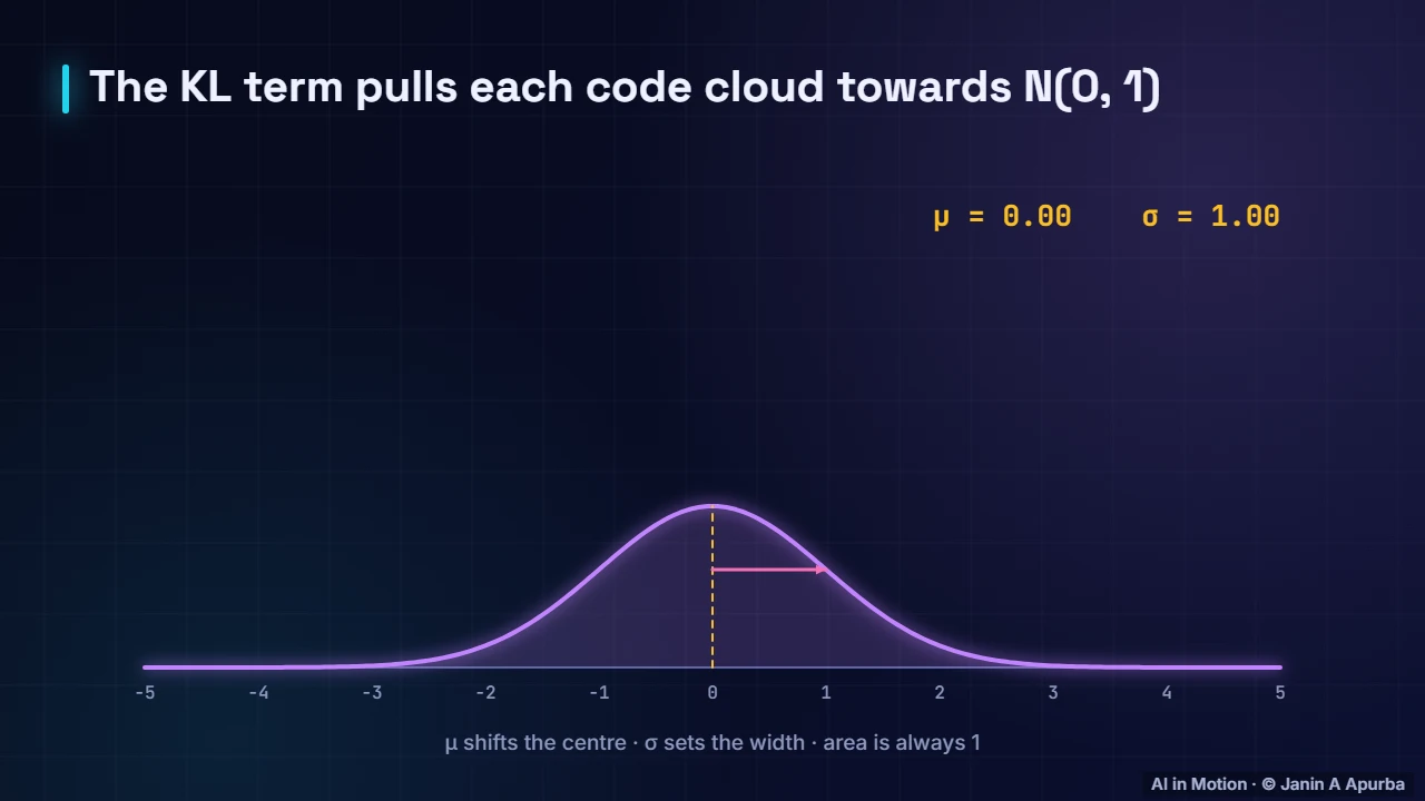
Here is the KL term at work on one input’s code cloud. It starts narrow and far from the centre. The penalty pulls its mean towards zero and its spread towards one, so that all the clouds overlap and together cover the standard normal, leaving no empty regions.
3:0910. The reparameterisation trick
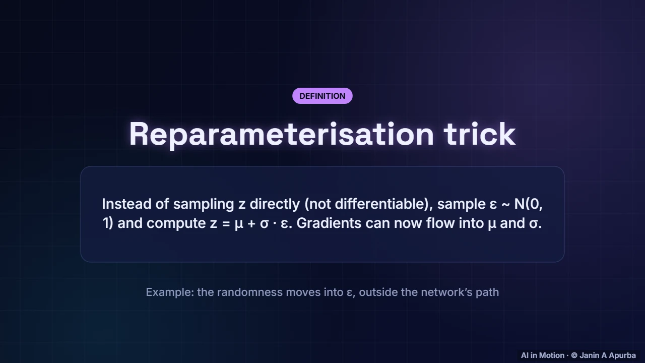
There is a technical obstacle: we cannot backpropagate through a random sampling step. The reparameterisation trick solves it. Sample plain noise epsilon from a standard normal, then compute the code as mu plus sigma times epsilon. The randomness now sits outside the path, and gradients flow into mu and sigma.
3:3011. Pause and think
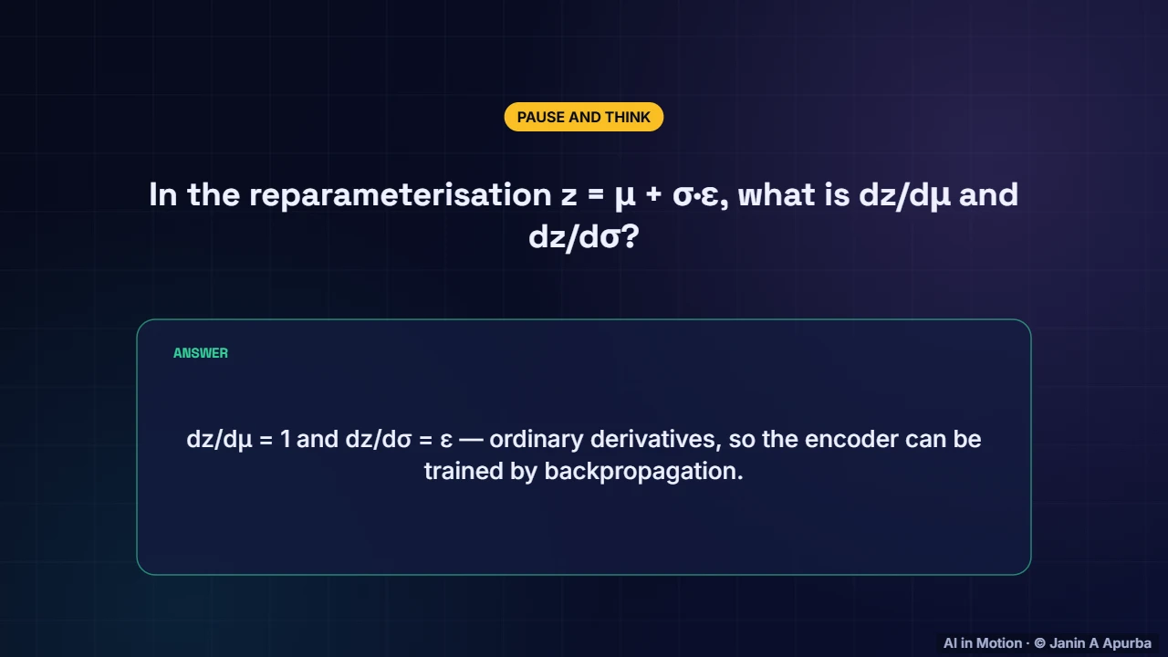
Pause and think. With z equal to mu plus sigma times epsilon, what are the derivatives of z with respect to mu and sigma? One, and epsilon. They are ordinary derivatives, which is exactly why the encoder can now be trained with backpropagation.
3:4812. A smooth latent space
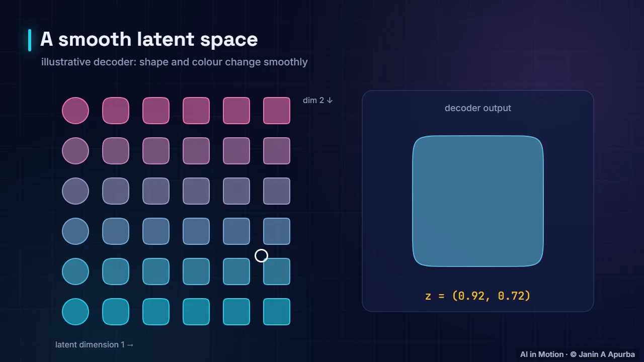
The payoff is a smooth latent space. Nearby codes decode to similar outputs. In this illustration, one direction changes the shape from circle to square, and the other changes the colour. Walking through the space morphs smoothly between them, and sampling any random point generates something new and sensible.
4:0913. The weakness
VAEs have a well known weakness: their samples tend to look blurry. With a pixel wise reconstruction loss, when several sharp details are plausible, the decoder hedges by outputting their average, which is a blur. VAEs therefore shine as compressors, for example inside Stable Diffusion, more than as final image makers.
4:3114. Disentangling factors
A simple variant, the beta VAE, weights the KL term more heavily. This pressure encourages each latent dimension to capture a single independent factor, such as one dimension for rotation and another for size, making the latent space easier to interpret, at some cost in reconstruction quality.
4:5115. Discrete codes
Another variant, the VQ VAE, replaces continuous codes with the nearest entry from a learned codebook, turning an image or a sound into a grid of discrete tokens. A transformer can then generate those tokens like words, an approach used by early text to image systems and many audio models.
5:1216. Generative adversarial networks
Generative adversarial networks, introduced by Ian Goodfellow and colleagues in 2014, take a completely different approach. Two networks compete. A generator turns random noise into fake samples, and a discriminator tries to tell real samples from fakes, like a counterfeiter against a detective. Each improves by beating the other.
5:3317. The adversarial game
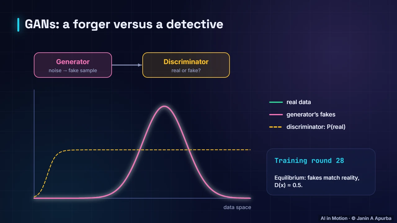
Here the green curve is real data and the pink curve is what the generator produces. At first its fakes are obviously wrong, and the discriminator, the dashed line, easily separates them. Round by round, the generator improves until its distribution matches the real one, and the discriminator can only guess, about fifty fifty.
5:5618. The minimax objective
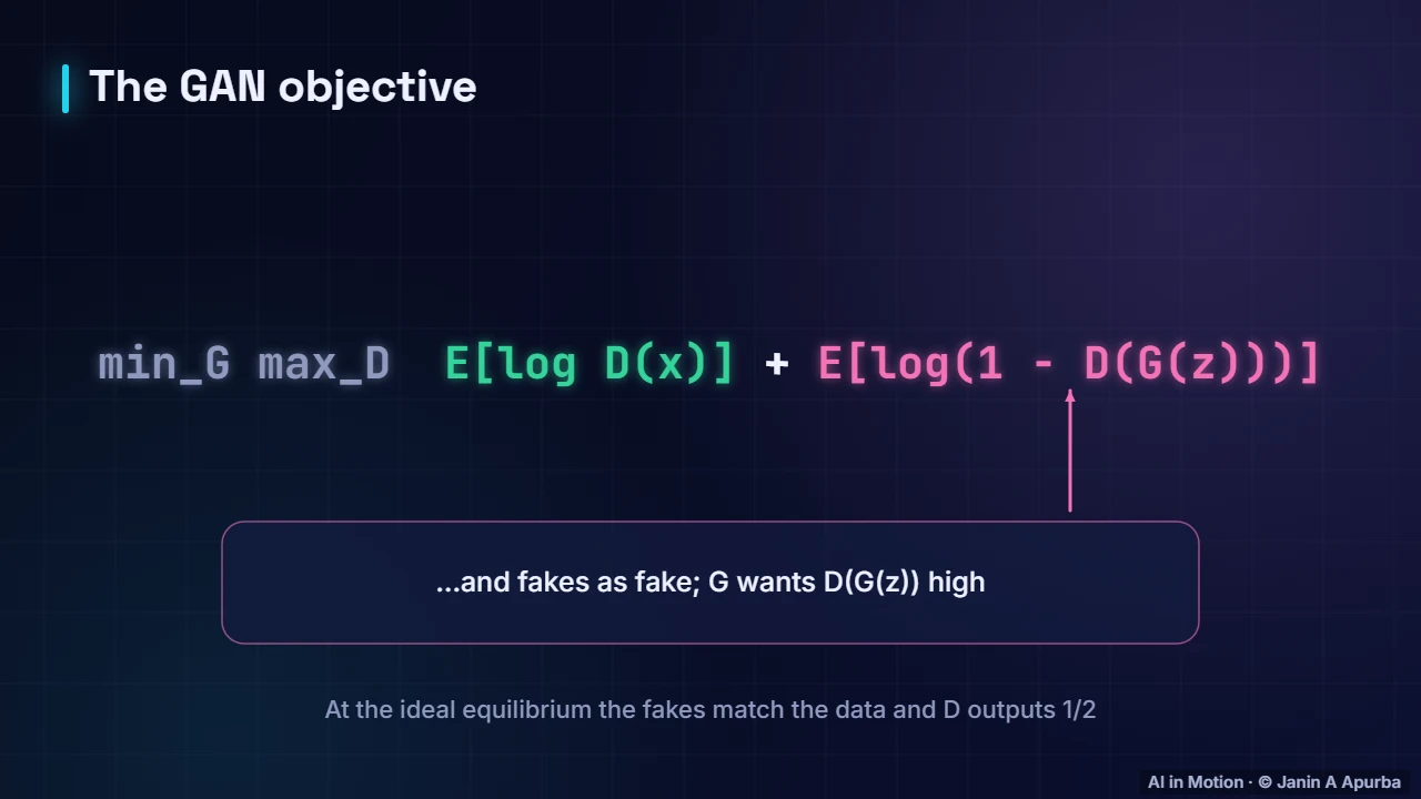
Formally, it is a minimax game. The discriminator maximises its log probability of labelling real data as real and fakes as fake. The generator minimises the same quantity, trying to make its fakes judged real. At the ideal equilibrium, the fake distribution matches the data, and the discriminator outputs one half everywhere.
6:1819. One training round
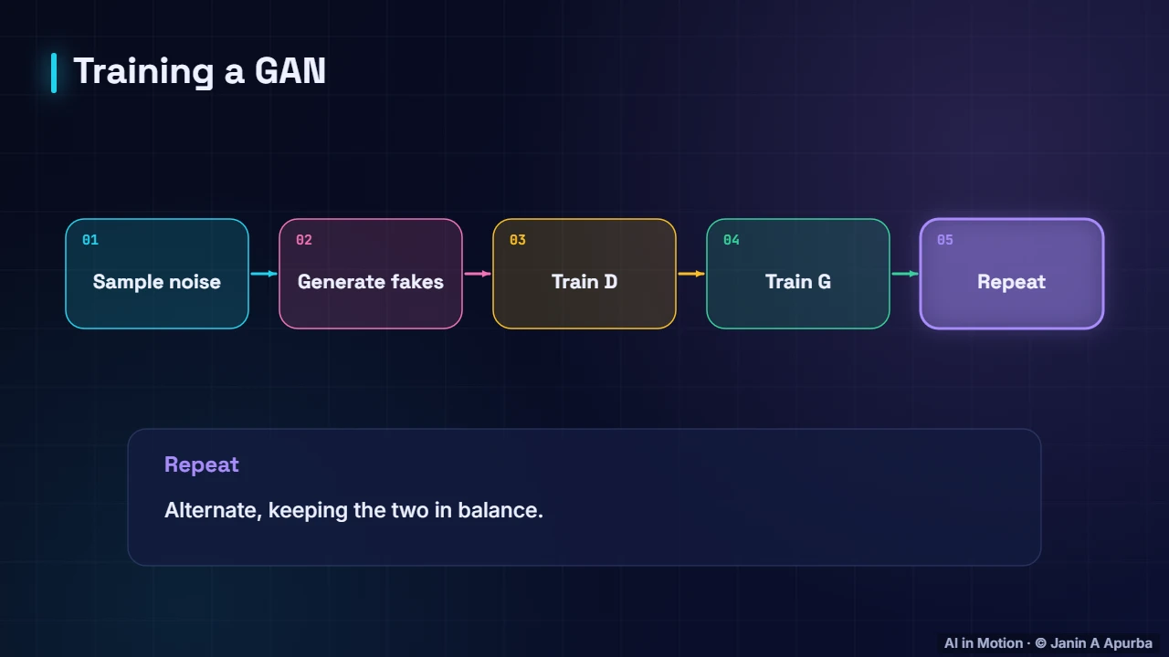
Training alternates. Sample random codes and let the generator produce fakes. Update the discriminator to label real samples as real and fakes as fake. Then update the generator so that the discriminator is fooled more often. Repeat, keeping the two players roughly in balance.
6:3720. Pause and think
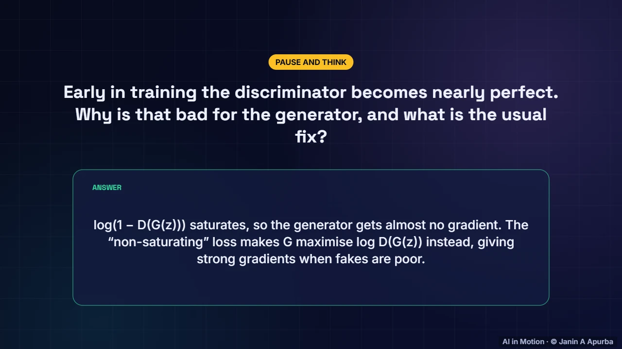
Pause and think. If the discriminator becomes nearly perfect early on, why is that bad for the generator? Its loss saturates, giving almost no gradient to learn from. The usual fix is the non saturating loss: the generator maximises the log of the discriminator’s score for its fakes instead.
6:5721. Mode collapse
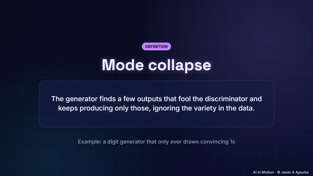
GANs suffer from mode collapse. The generator discovers a few outputs that reliably fool the discriminator and produces only those, ignoring the rest of the data’s variety. A handwritten digit generator might draw only very convincing ones. Detecting and preventing this was a major research topic.
7:1722. Stabilising GANs
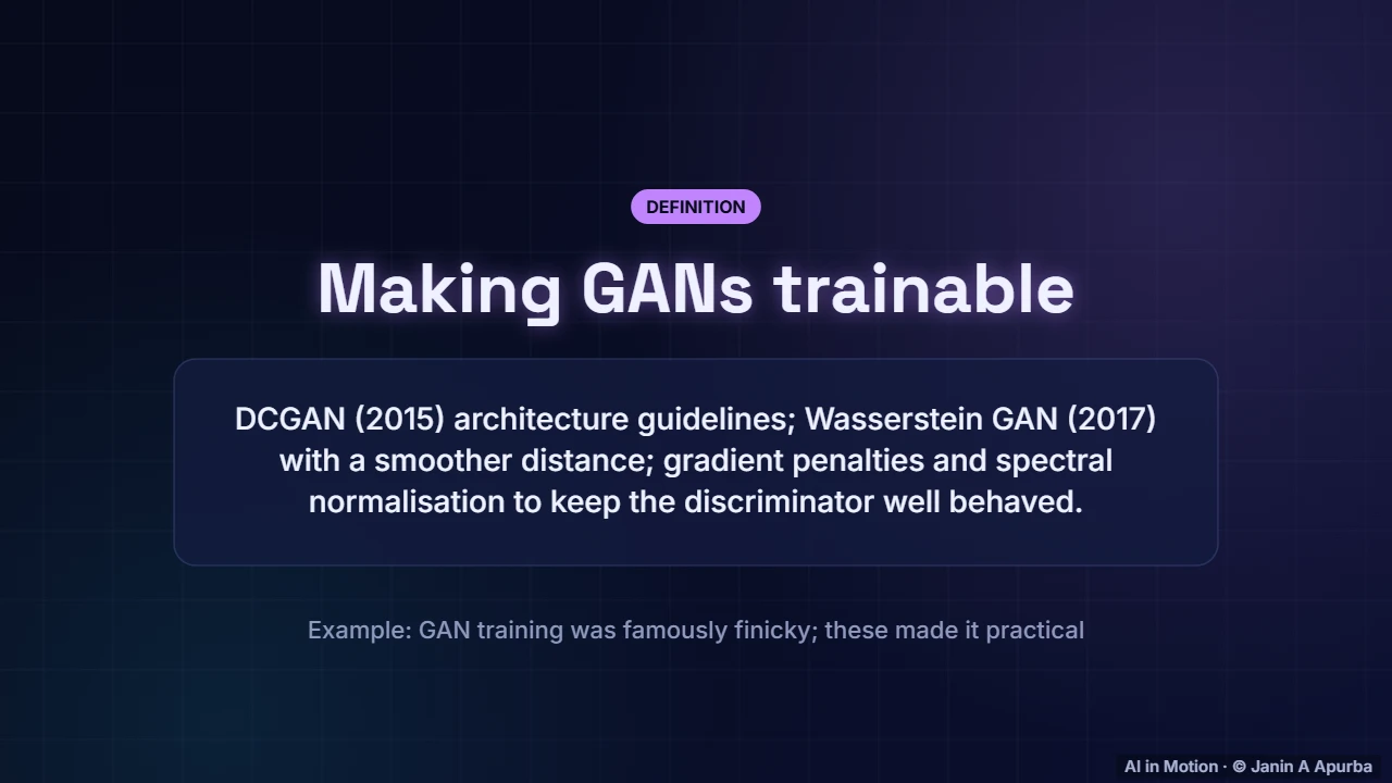
Several advances made GANs practical. DCGAN, in 2015, gave convolutional architecture guidelines that trained reliably. The Wasserstein GAN, in 2017, replaced the original objective with a smoother distance between distributions, and gradient penalties and spectral normalisation kept the discriminator well behaved.
7:3523. GAN milestones
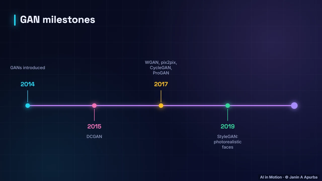
The field moved fast. GANs appeared in 2014 and DCGAN in 2015. 2017 brought the Wasserstein GAN, image to image translation with pix two pix and CycleGAN, and progressive growing. StyleGAN produced photorealistic faces in 2019, and by 2021 diffusion models overtook GANs on standard quality benchmarks.
7:5524. Conditional GANs
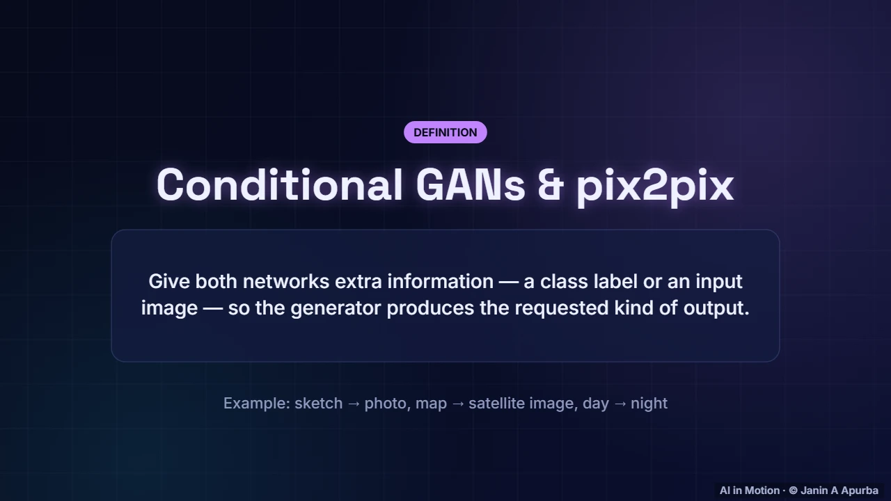
Conditional GANs give both networks extra information, such as a class label or an input image, so the generator produces what is requested. Pix two pix, from 2017, learned image to image translation from paired examples: sketches to photos, maps to satellite images, day scenes to night.
8:1525. CycleGAN
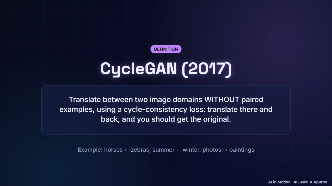
CycleGAN went further, translating between two domains without any paired examples. Its trick is cycle consistency: translate a horse photo into a zebra and back again, and you should recover the original horse. It turned summer scenes into winter and photographs into paintings.
8:3326. StyleGAN
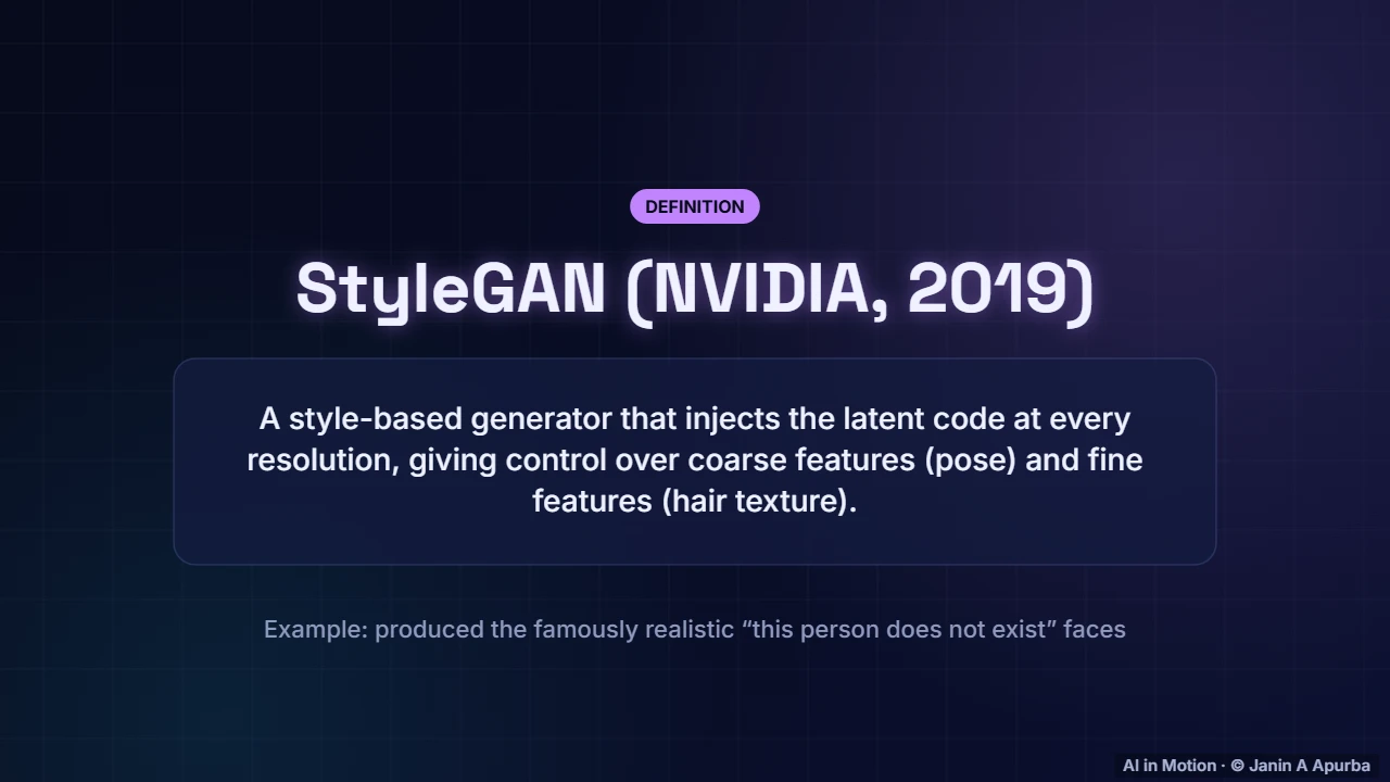
StyleGAN, from NVIDIA in 2019, injected the latent code at every resolution of the generator. Coarse layers controlled pose and face shape, and fine layers controlled texture and colour. It produced strikingly realistic faces of people who do not exist, and made the risks of synthetic media obvious.
8:5427. Evaluating generators
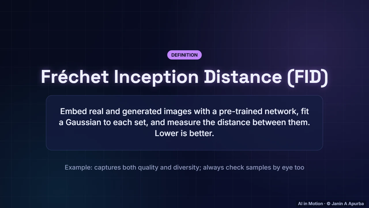
How do we score a generator? The Fréchet Inception Distance embeds real and generated images with a pre trained image network, fits a Gaussian to each set of embeddings, and measures the distance between the two. Lower is better, and it captures both quality and diversity, though human inspection is still essential.
9:1628. VAE vs GAN vs diffusion
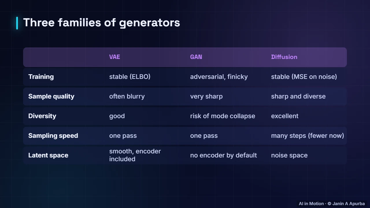
Here is the comparison. VAEs train stably and have smooth latent spaces with an encoder, but samples are often blurry. GANs produce very sharp images in a single pass, but training is finicky and diversity can collapse. Diffusion models train stably and give sharp, diverse samples, at the cost of many sampling steps.
9:3829. Pause and think
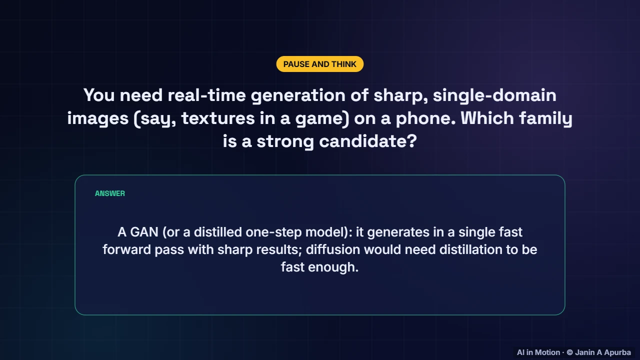
Pause and think. You need real time generation of sharp images from one domain, such as game textures, on a phone. Which family is a strong candidate? A GAN, or a distilled one step model, because it generates sharp results in a single fast pass. Standard diffusion would be too slow without distillation.
10:0030. A GAN step in code
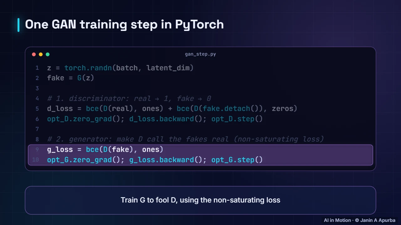
One GAN step in PyTorch has two halves. Sample noise and generate fakes. Train the discriminator with binary cross entropy, labelling real as one and fake as zero, detaching the fakes so the generator is not updated. Then train the generator to make the discriminator call its fakes real.
10:2131. Uses and risks
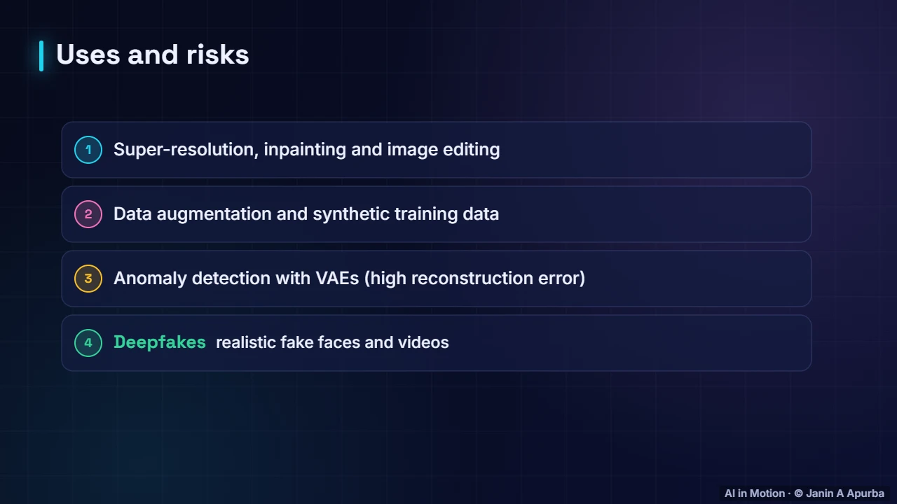
These models have many uses: super resolution, inpainting and editing, synthetic training data and augmentation, and anomaly detection, where a VAE flags inputs it cannot reconstruct well. They also enabled deepfakes, realistic fake faces and videos, which is why detection and provenance tools matter.
10:4032. Recap
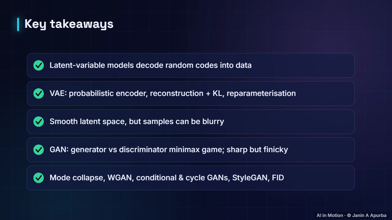
To recap. Both families decode random codes into data. VAEs use a probabilistic encoder, a reconstruction plus KL loss and the reparameterisation trick, giving smooth latent spaces but blurrier samples. GANs pit a generator against a discriminator, giving sharp samples but finicky training, with mode collapse as the classic failure.
Key takeaways
- VAEs and GANs are latent-variable models that decode random codes into data.
- A VAE’s encoder outputs μ and σ; the loss is reconstruction + KL(q(z|x) ‖ N(0, I)), the negative ELBO.
- The reparameterisation trick z = μ + σ·ε makes sampling differentiable.
- GANs train a generator and a discriminator in a minimax game; at equilibrium D outputs ½.
- GAN pitfalls: vanishing generator gradients (use the non-saturating loss) and mode collapse; WGAN and spectral normalisation stabilise training.
- Conditional GANs, pix2pix, CycleGAN and StyleGAN extended GANs; FID measures sample quality and diversity.
Check yourself
- What does a VAE encoder output for each input?
Show answer
A mean and a spread (a distribution over codes) — Codes are probability clouds.
- What does the reparameterisation trick achieve?
Show answer
Differentiable sampling via z = μ + σ·ε — Randomness moves into ε.
- At the ideal GAN equilibrium, the discriminator outputs…
Show answer
½ everywhere — Fakes are indistinguishable from real data.
- What is mode collapse?
Show answer
The generator produces only a few kinds of outputs — Diversity is lost.
- Which family typically produces blurrier samples?
Show answer
VAEs — Pixel-wise likelihood averages plausible details.
Go deeper
- Variational Autoencoders: Probabilistic Latent Spaces · The AI Lecture Hall
- Generative Adversarial Networks: The Generator–Discriminator Game · The AI Lecture Hall
- GAN Variants: Conditional GANs, Pix2Pix, CycleGAN and StyleGAN · The AI Lecture Hall
- Autoencoders: Compression, Denoising and Representation Learning · The AI Lecture Hall
- Generative vs Discriminative Models: Learning to Create · The AI Lecture Hall
© 2026 Janin A Apurba, CSE, AUST · Advanced ICT Officer, CNRS-UNHCR. All rights reserved. Notes for the animated lecture at https://ai-in-motion.vercel.app/watch/gans-and-vaes-deep-dive.html