From RNNs to Transformers: Sequence Models in Depth — lecture notes
How neural networks learned to handle sequences: recurrent networks and backpropagation through time, vanishing gradients, LSTM and GRU gates, encoder–decoder translation, attention, and why transformers replaced recurrence.
0:001. Introduction
Language, speech, music, sensor readings and stock prices all arrive as sequences, where order matters. In this deep dive we follow the story of sequence models: recurrent networks, their memory problems, the gated LSTM and GRU, attention, and finally the transformer, which now powers most of modern AI.
0:202. Sequence data
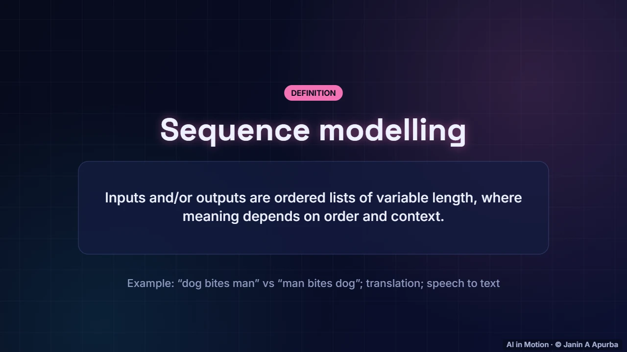
Sequence modelling deals with ordered data of variable length, where meaning depends on order and context. Dog bites man and man bites dog use the same words but mean very different things. Translation, speech recognition and forecasting are all sequence problems.
0:383. Why ordinary networks struggle
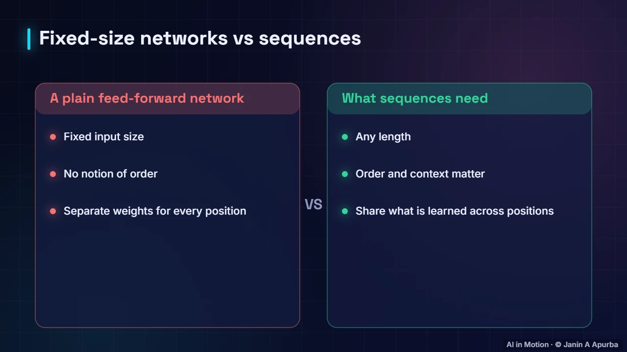
A plain feed forward network expects a fixed number of inputs, has no built in sense of order, and would need separate weights for every position. Sequences need models that handle any length, respect order and context, and reuse what they learn at one position everywhere else.
0:584. Recurrent neural networks
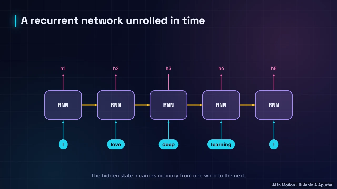
A recurrent neural network reads a sequence one step at a time. At each step it combines the current word with its hidden state, a memory of everything read so far, and produces a new hidden state. The same weights are reused at every step, so it handles sequences of any length.
1:205. The RNN update
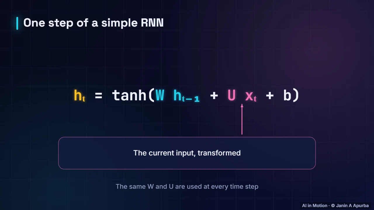
Mathematically, the new hidden state is tanh of the previous state times a matrix W, plus the current input times a matrix U, plus a bias. Crucially, the same W and U are used at every time step, which is what lets one small set of weights process sequences of any length.
1:426. Training RNNs
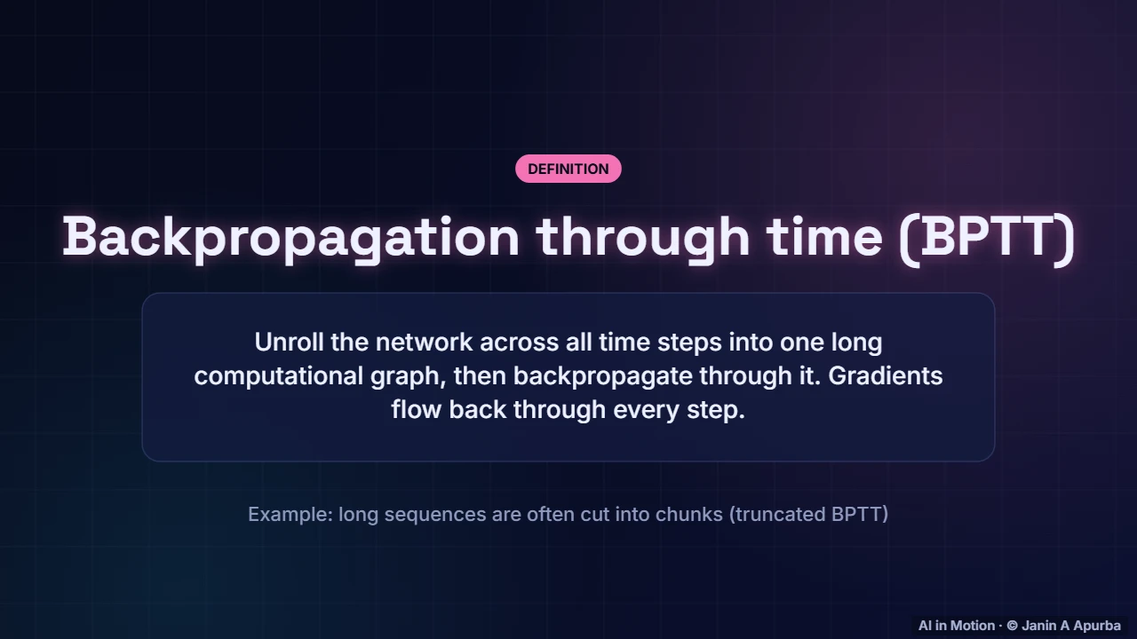
To train a recurrent network, we unroll it across all time steps, turning it into one long computational graph, and then backpropagate through it. This is called backpropagation through time. For long sequences, the unrolled graph is often cut into chunks to save memory.
2:007. Vanishing through time
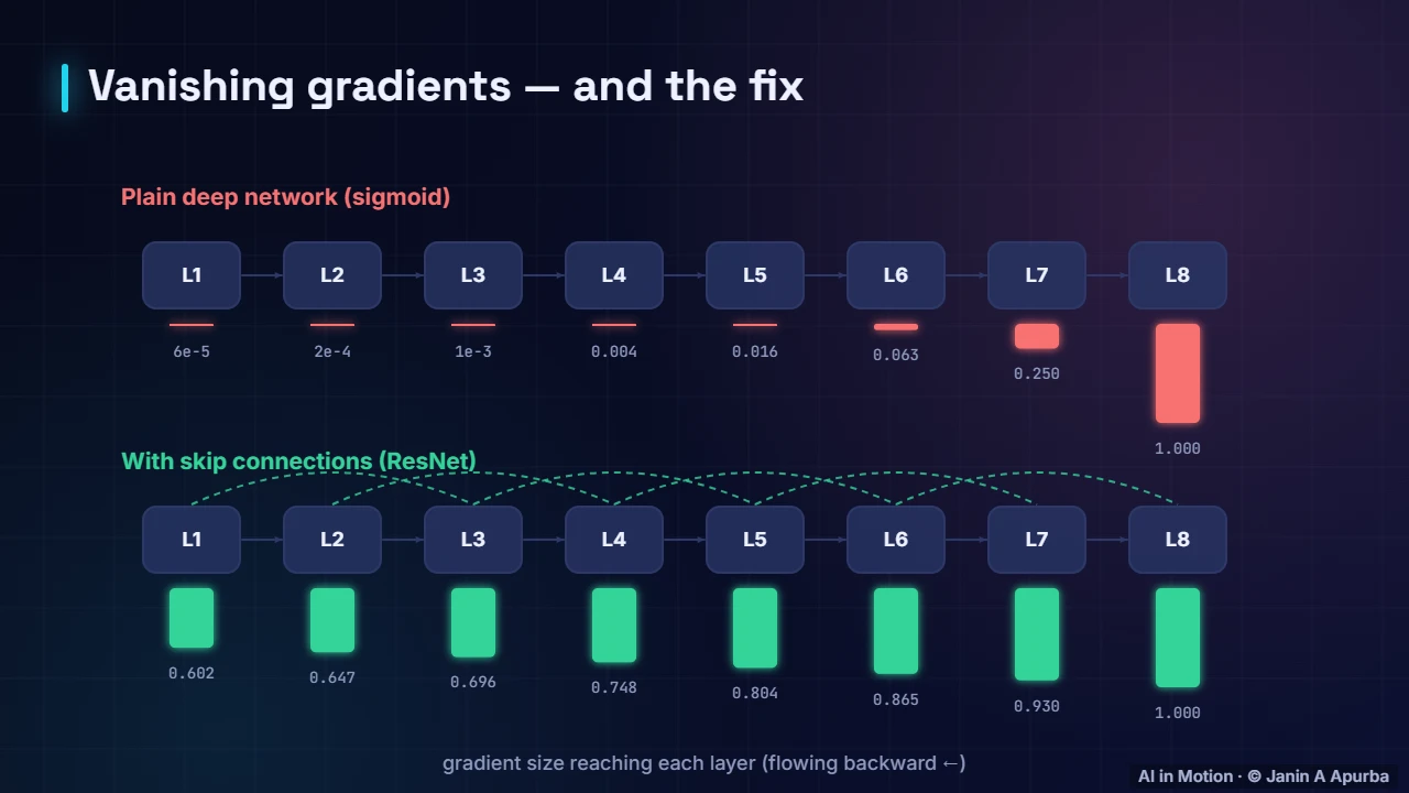
Unrolling reveals a problem. The gradient reaching early time steps is a product of many local slopes, one per step. If those are mostly below one, the product shrinks towards zero, just as in a deep sigmoid network. Here, after eight steps almost nothing is left, so early words barely influence learning.
2:228. Pause and think
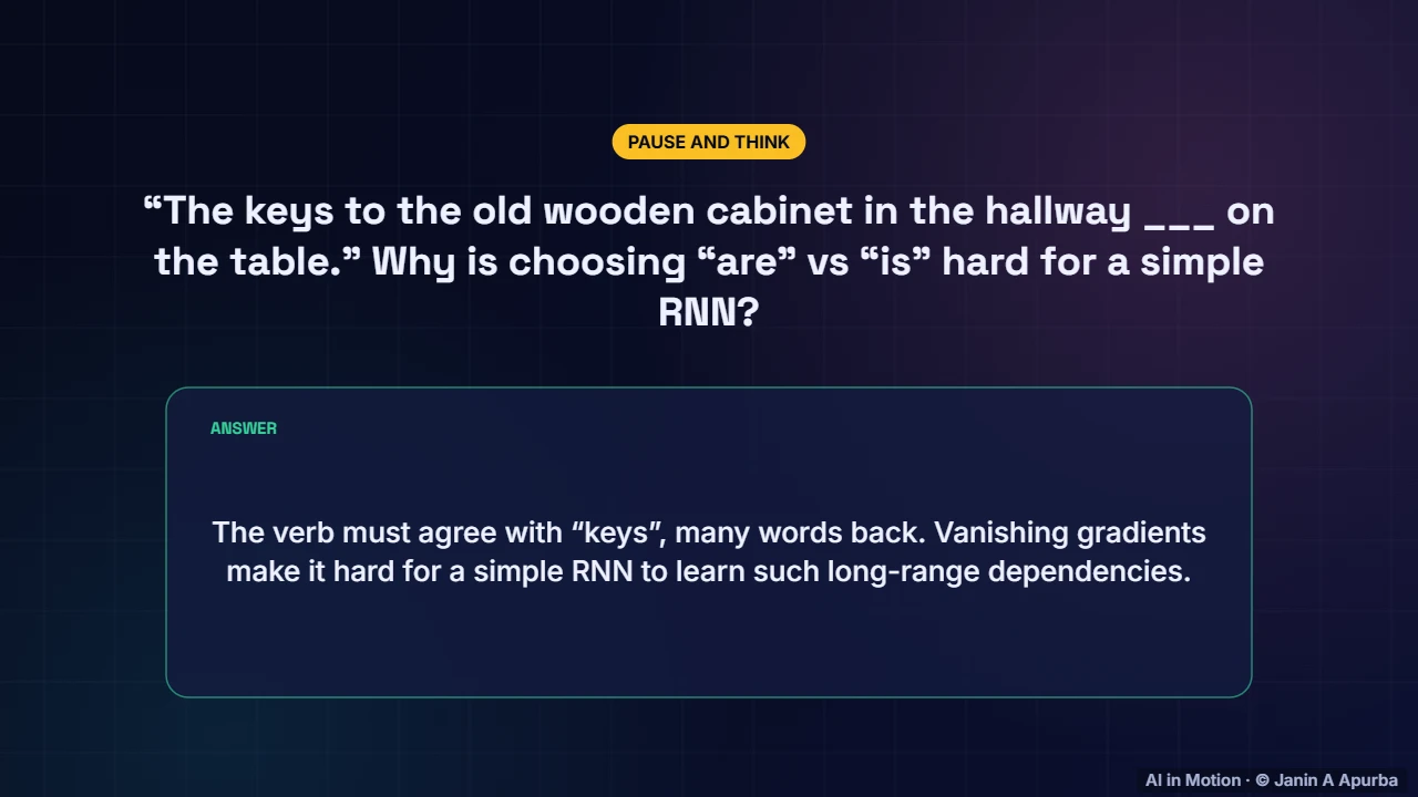
Pause and think. The keys to the old wooden cabinet in the hallway, blank, on the table. Why is choosing are or is hard for a simple RNN? The verb must agree with keys, many words earlier, and vanishing gradients make such long range dependencies very hard to learn.
2:439. The LSTM
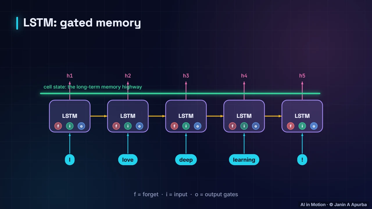
The long short term memory network, the LSTM, solved this in 1997. It adds a cell state, a memory highway running along the top, and three gates. The forget gate decides what to erase, the input gate decides what new information to store, and the output gate decides what to reveal.
3:0510. The cell state
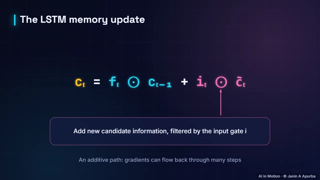
The key equation is additive. The new cell state keeps a gated fraction of the old one, plus a gated amount of new information. Because memory is carried forward by addition rather than repeated multiplication, gradients can flow back through many time steps without vanishing.
3:2411. The GRU
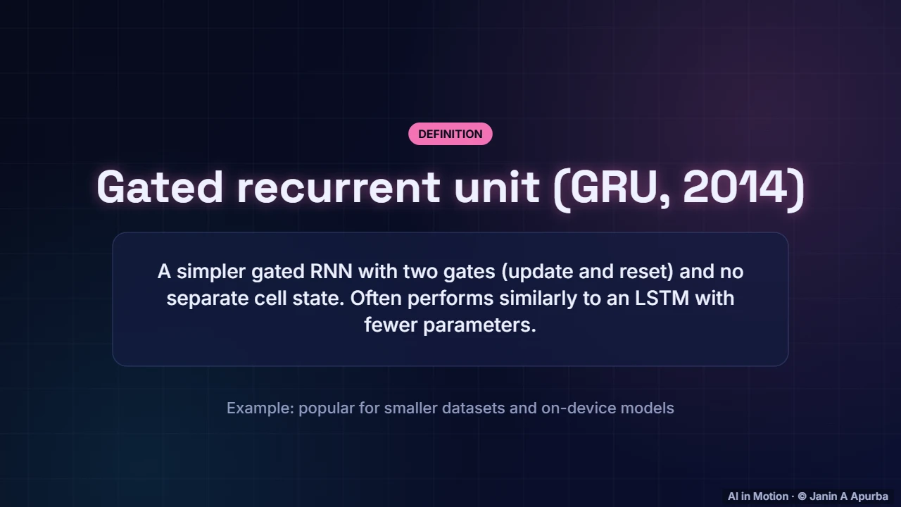
The gated recurrent unit, introduced in 2014, is a streamlined alternative. It merges the cell and hidden states and uses just two gates, update and reset. With fewer parameters it trains a little faster, and on many tasks it performs about as well as an LSTM.
3:4412. Recurrent cells compared
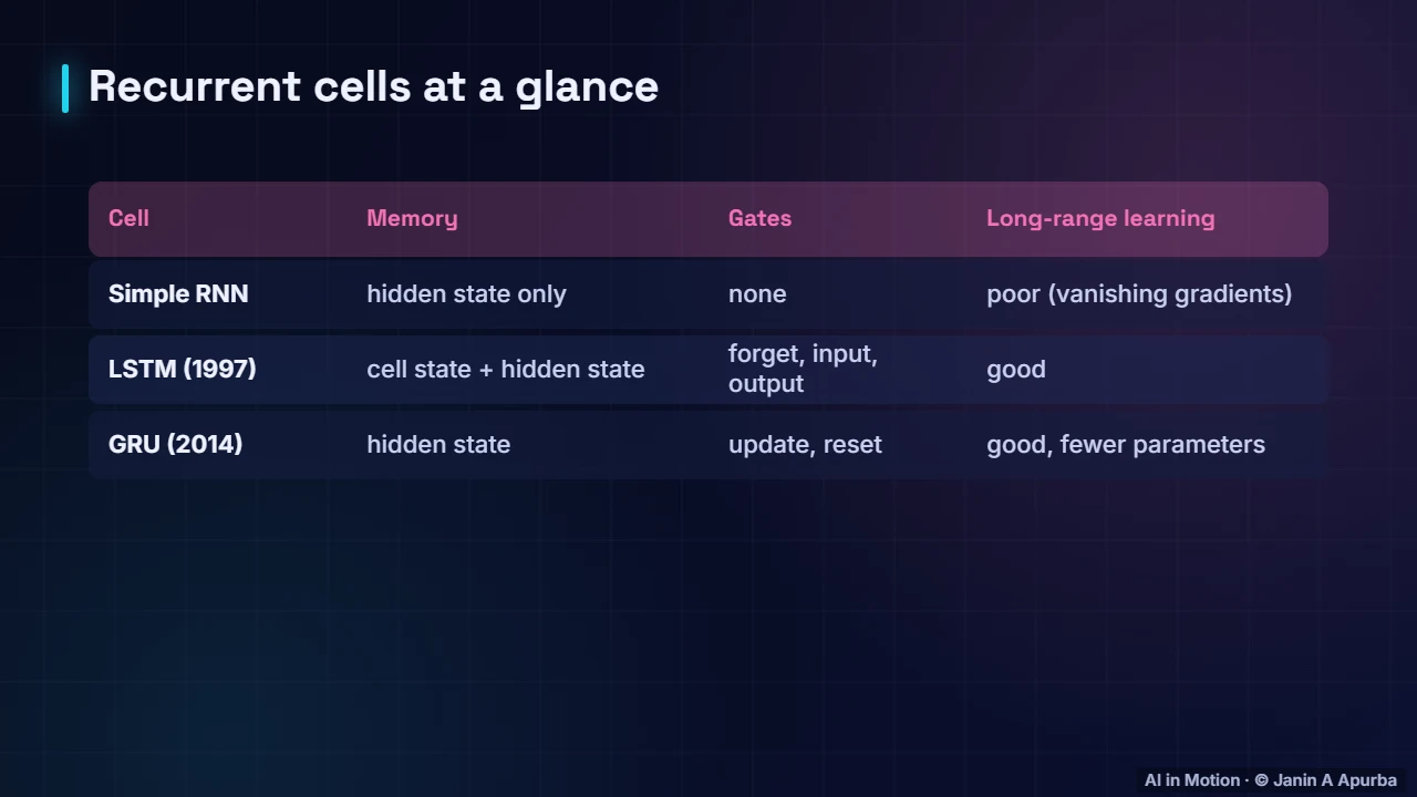
In summary, a simple RNN has only its hidden state and struggles with long range dependencies. The LSTM adds a cell state and three gates and learns long range patterns well. The GRU achieves similar results with two gates and fewer parameters.
4:0213. Bidirectional RNNs
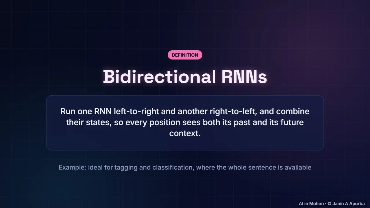
When the whole sequence is available in advance, as in tagging words or classifying a review, we can read it both ways. A bidirectional RNN runs one network left to right and another right to left, and combines their states, so every position benefits from both earlier and later context.
4:2314. Encoder–decoder translation
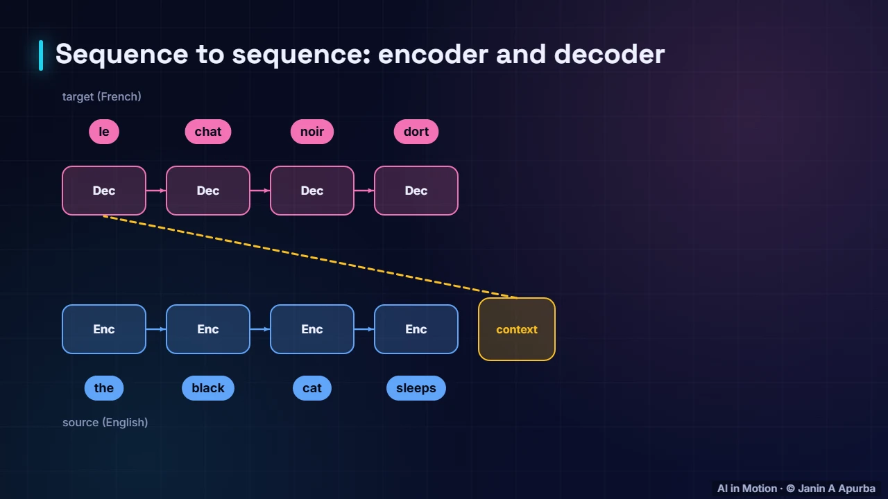
In 2014, recurrent networks transformed machine translation with the encoder decoder design. The encoder reads the English sentence and compresses it into a context vector. The decoder then writes the French translation one word at a time: le chat noir dort. Notice the word order changes.
4:4315. Teacher forcing
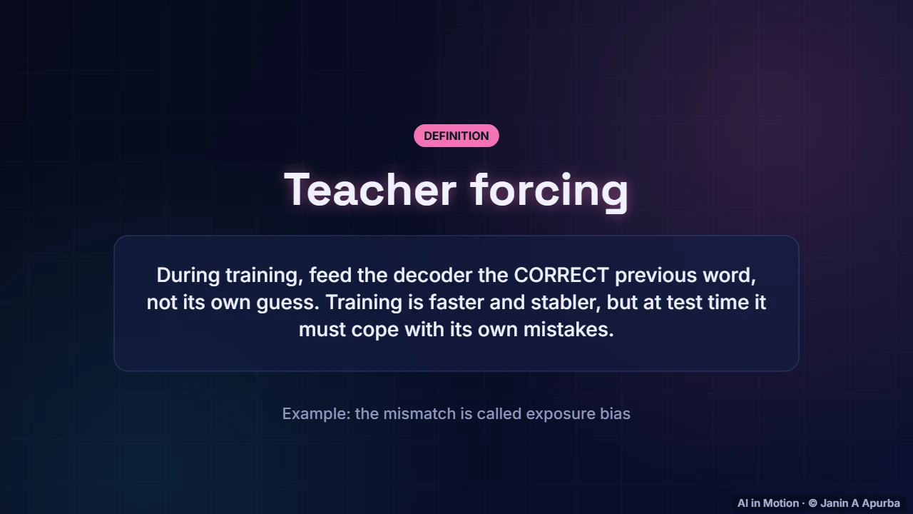
How is the decoder trained? With teacher forcing: at each step it receives the correct previous word from the reference translation, rather than its own guess. This makes training fast and stable. At test time, however, it must build on its own outputs, and that mismatch is known as exposure bias.
5:0416. Beam search
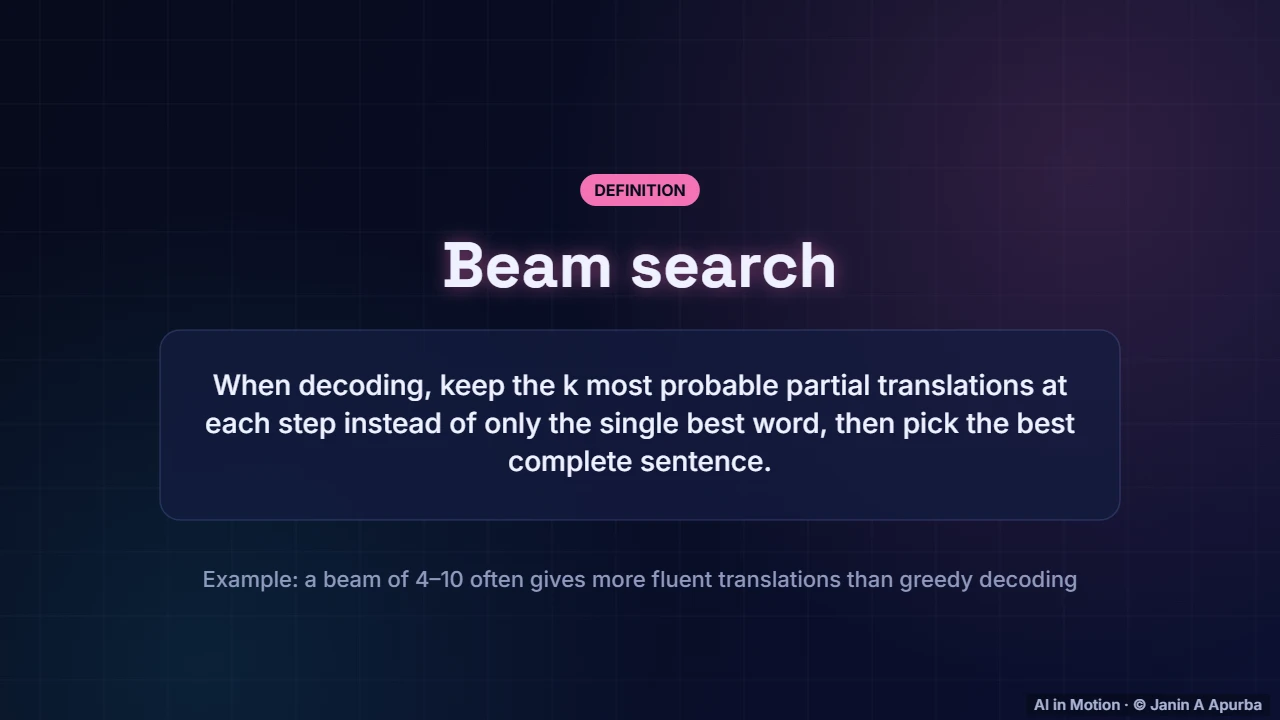
When generating a translation, always taking the single most likely next word can paint the decoder into a corner. Beam search keeps the k most probable partial sentences at every step, expands each of them, and finally picks the best complete sentence. Beams of four to ten are common in translation.
5:2617. The bottleneck
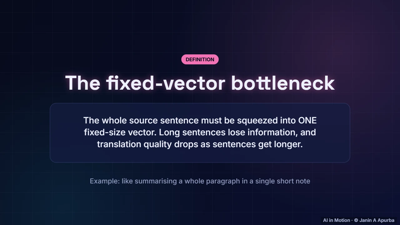
There was a bottleneck. The entire source sentence had to be squeezed into one fixed size vector, like summarising a paragraph on a sticky note. Short sentences survived, but as sentences grew longer, information was lost and translation quality fell.
5:4318. Attention
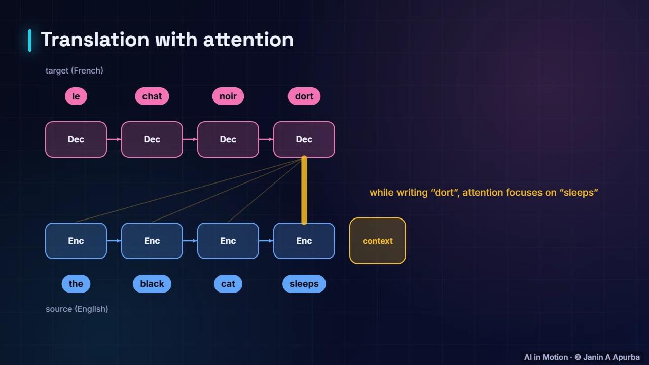
Attention removed the bottleneck. At every output step, the decoder looks back at all of the encoder’s states and decides which to focus on. When writing chat, it attends to cat. When writing noir, it attends to black. The word order problem solves itself, and long sentences translate far better.
6:0419. Attention weights
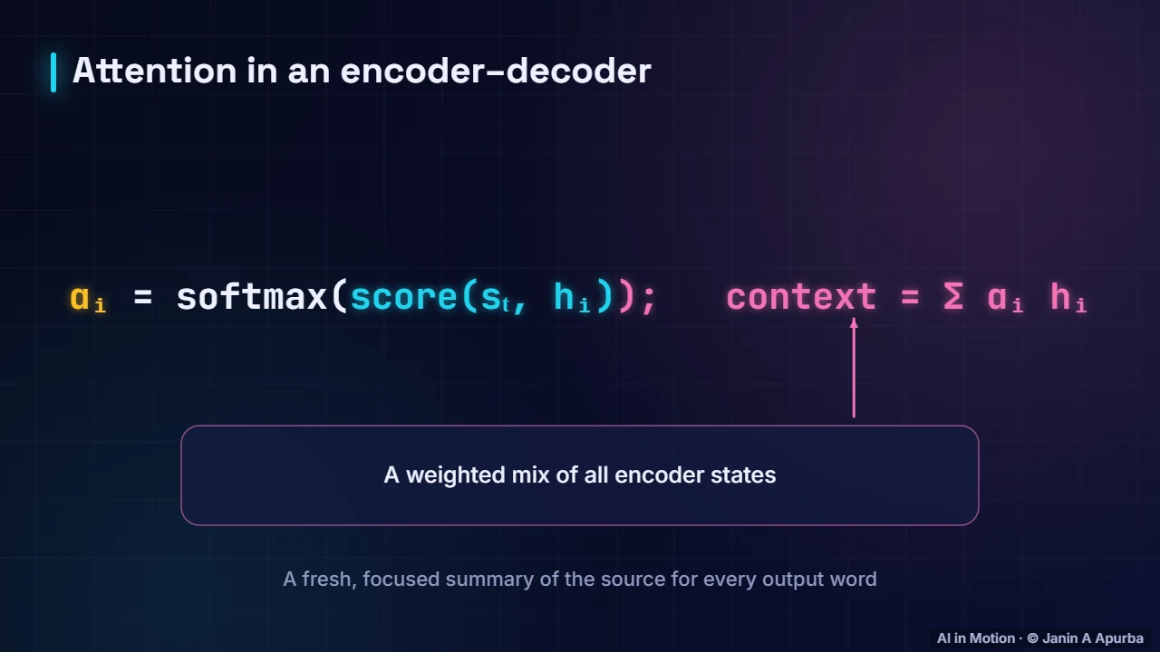
Mechanically, the decoder scores how relevant each encoder state is to its current state, turns the scores into weights with a softmax, and builds a context vector as the weighted sum of the encoder states. Every output word gets its own fresh, focused summary of the source sentence.
6:2520. Pause and think
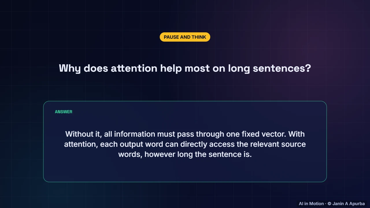
Pause and think. Why does attention help most on long sentences? Without it, everything must pass through a single fixed vector, which overflows. With attention, each output word reaches directly into the relevant source words, however long the sentence is.
6:4221. The transformer
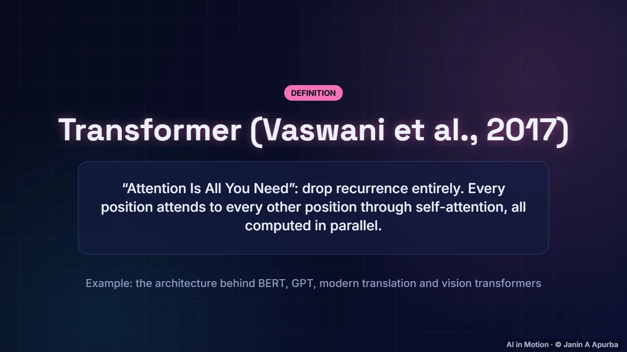
In 2017, the paper Attention is all you need asked a bold question: what if we drop recurrence entirely? The transformer processes all positions at once, and every word attends directly to every other word through self attention. It became the architecture behind BERT, GPT and most modern AI.
7:0322. Self-attention
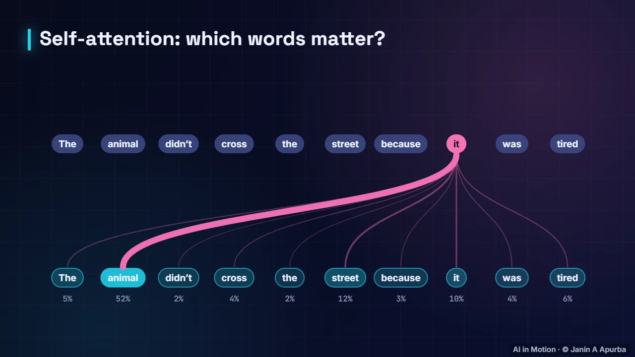
Read this sentence: the animal did not cross the street because it was tired. What does it refer to? Self attention lets the word it look at every other word and assign weights. Here most of its attention goes to animal, exactly the right answer, found in a single step.
7:2423. Queries, keys and values
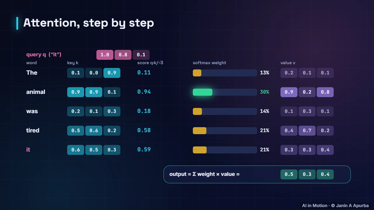
Under the hood, each word emits a query, a key and a value. The query for it is compared with every key by a dot product, scaled and passed through a softmax. The animal receives the largest weight, and the output is the weighted mix of the values.
7:4524. Masks
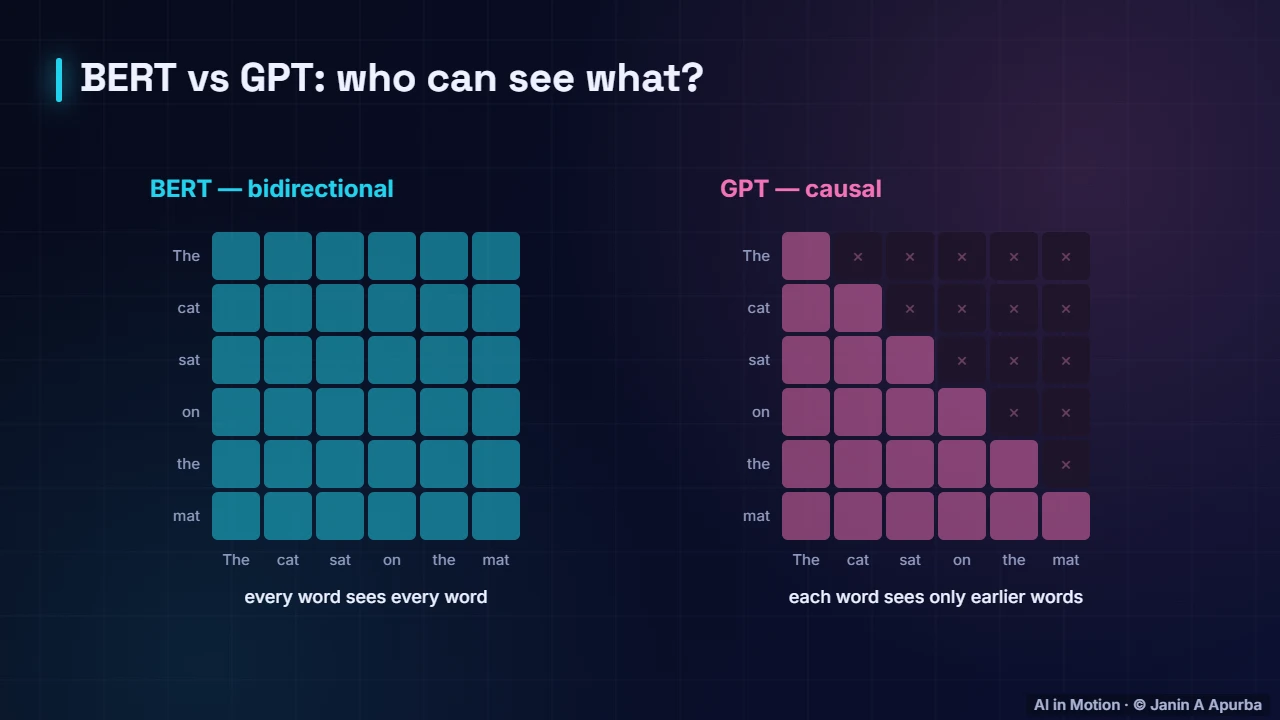
Transformers control what each word may see with attention masks. In an encoder like BERT, every word attends to every other word. In a decoder like GPT, a causal mask blocks the future, so each word sees only earlier words and the model can be trained to predict the next one.
8:0625. Order without recurrence
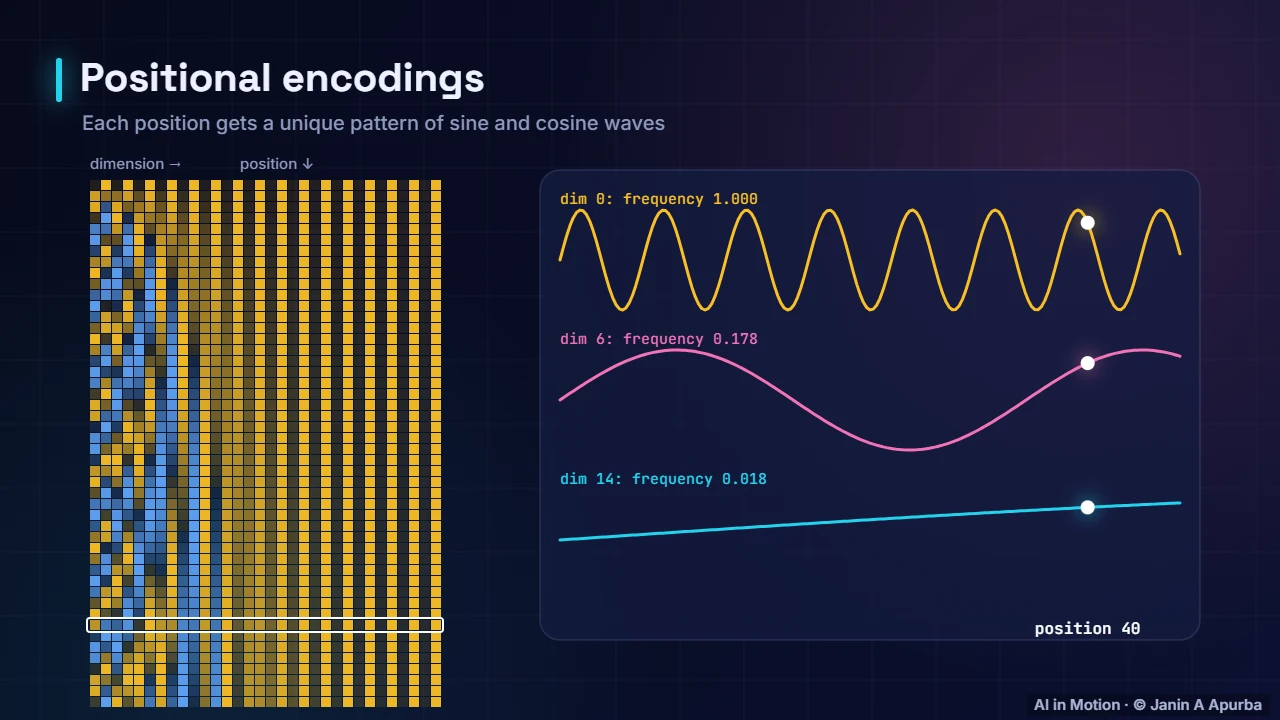
Without recurrence, a transformer has no built in sense of order, so position information is added to each word’s embedding. The original transformer used sine and cosine waves of different frequencies, giving every position a unique fingerprint. Modern models often rotate queries and keys instead.
8:2526. The full architecture
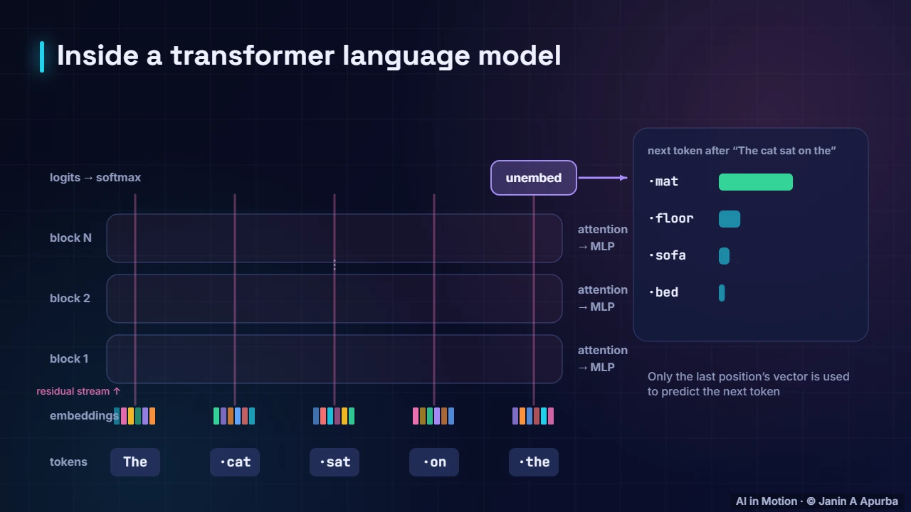
Here is a decoder only transformer in full. Tokens become embeddings, which flow up through a stack of identical blocks, each combining self attention with a small feed forward network, connected by residual paths. The final vector predicts the next token.
8:4327. RNN vs transformer
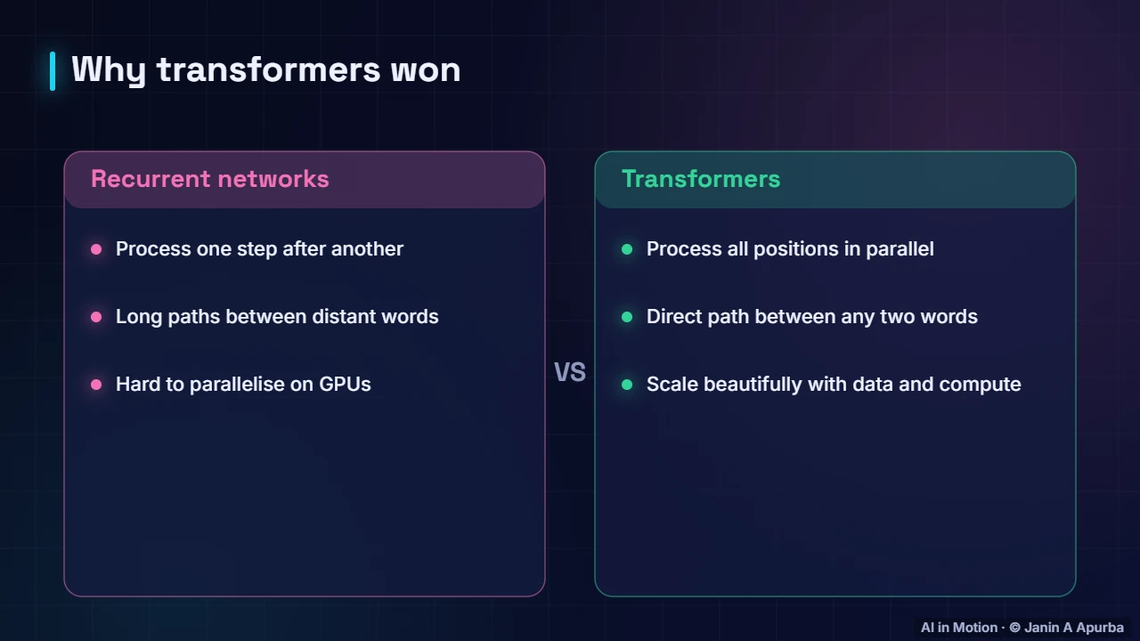
Why did transformers win? Recurrent networks must process one step after another, so training cannot be parallelised across the sequence, and information between distant words travels a long path. Transformers process all positions in parallel on GPUs and connect any two words directly, and they scale remarkably well with data and compute.
9:0528. The price
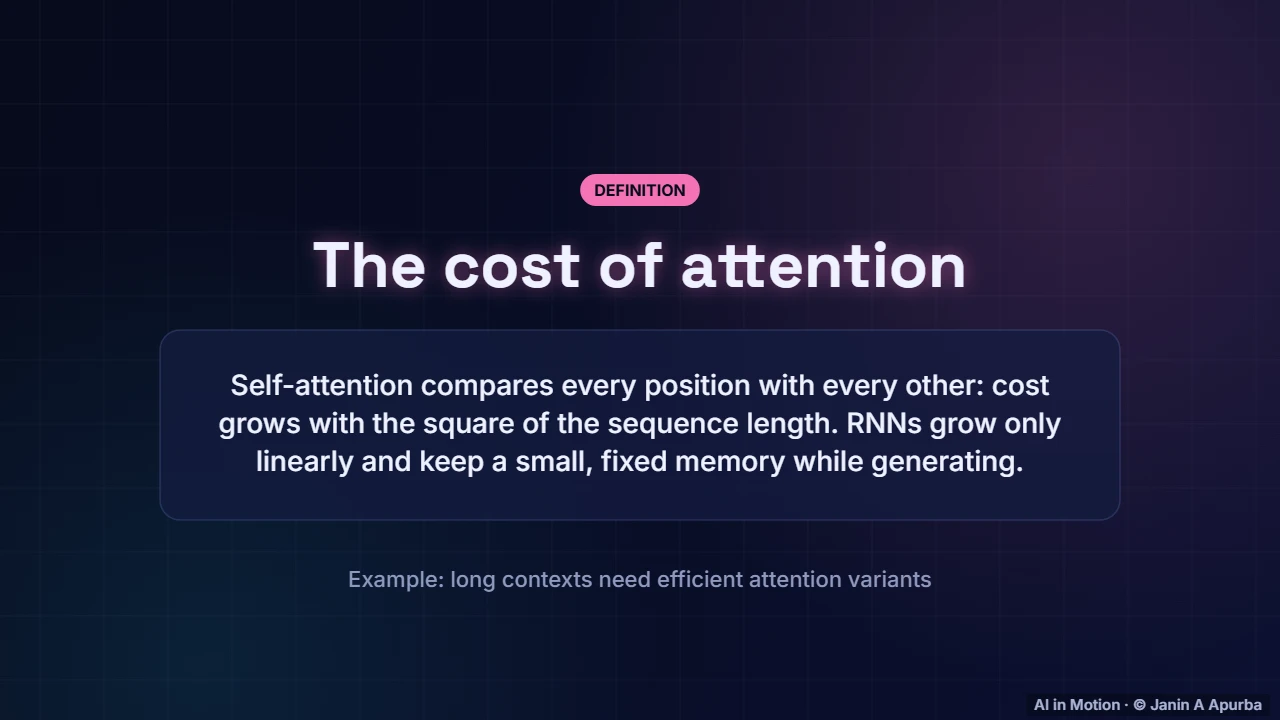
Transformers do pay a price. Self attention compares every position with every other, so its cost grows with the square of the sequence length. Recurrent networks grow only linearly and keep a small fixed memory while generating, which is why efficient attention variants are an active research area.
9:2529. The comeback
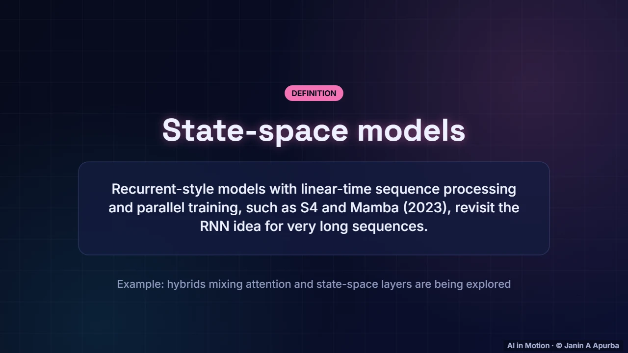
Interestingly, recurrence is making a comeback. State space models such as S four and Mamba, from 2023, process sequences in linear time like an RNN, yet can be trained in parallel. Hybrid models that mix attention layers with state space layers are being actively explored for very long sequences.
9:4630. The journey
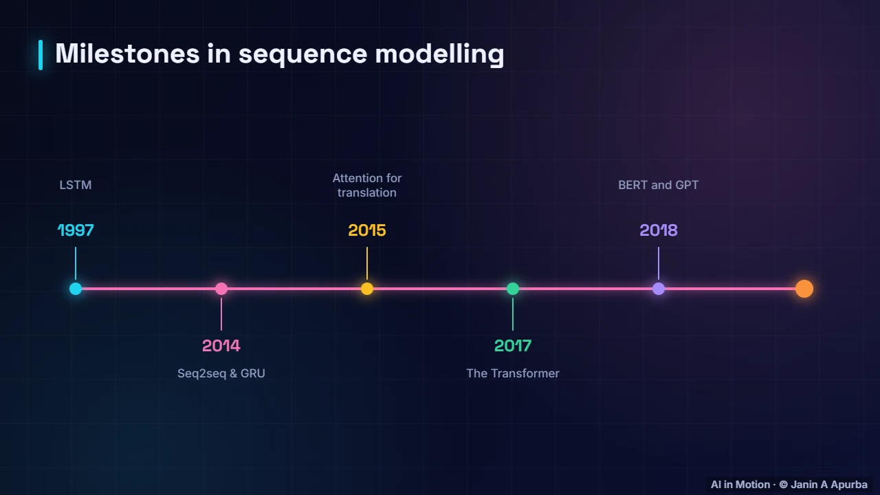
Here is the journey. The LSTM appeared in 1997. Encoder decoder models and the GRU arrived in 2014, and attention transformed translation around 2015. The transformer followed in 2017, BERT and GPT in 2018, and state space models such as Mamba in 2023.
10:0531. Pause and think
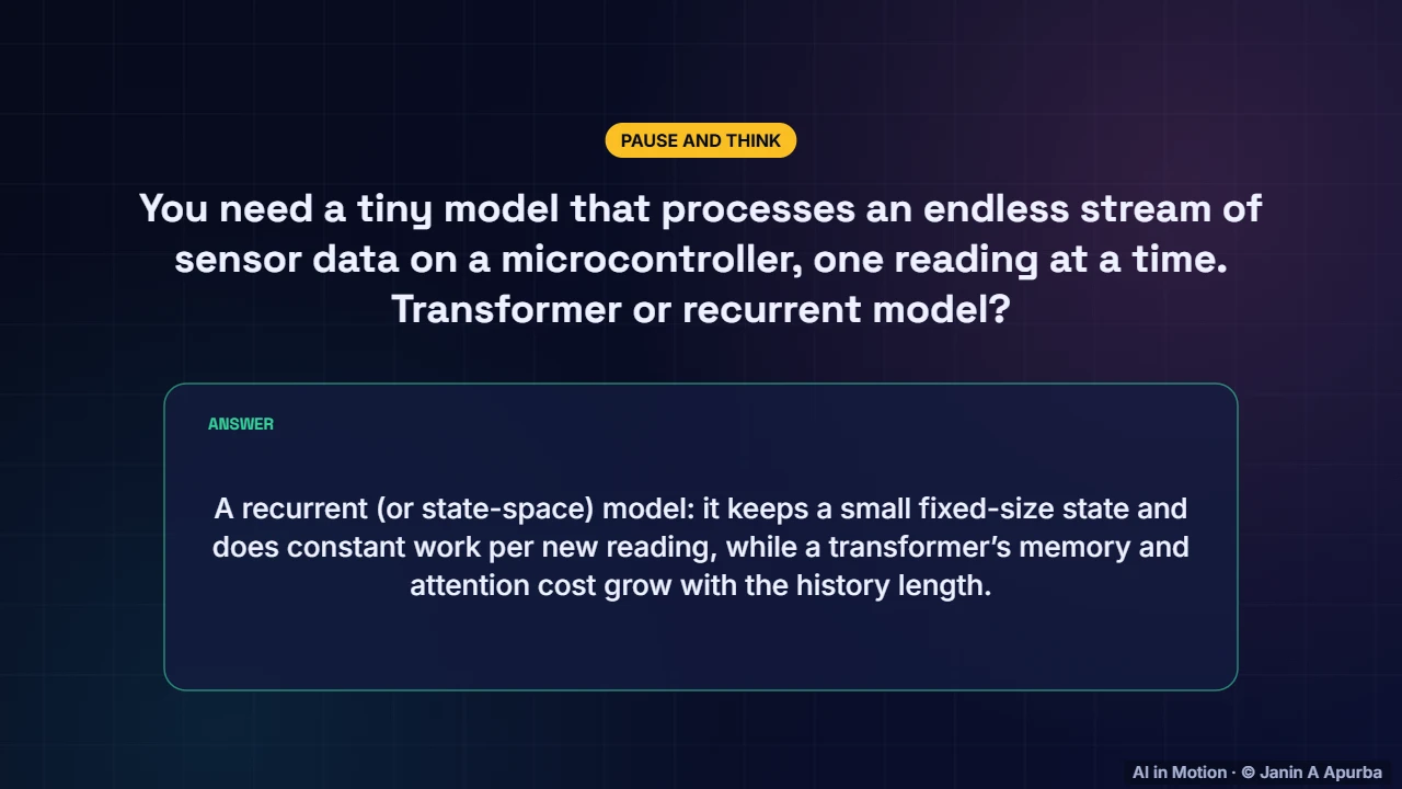
Pause and think. You need a tiny model that processes an endless stream of sensor readings on a microcontroller, one at a time. Transformer or recurrent model? A recurrent or state space model, which keeps a small fixed state and does constant work per reading, while attention cost grows with history.
10:2632. In code
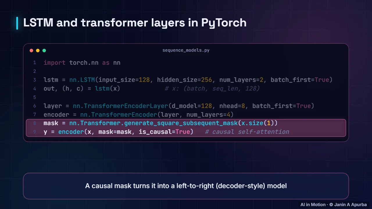
Both families are a few lines in PyTorch. An LSTM layer returns its outputs plus the final hidden and cell states. A transformer encoder stacks layers with multi head self attention, and adding a causal mask makes it read strictly left to right, like a GPT style decoder.
10:4733. Recap
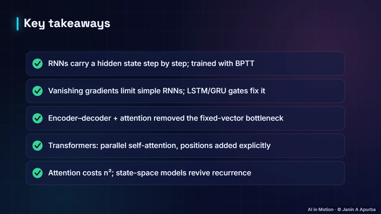
To recap. Recurrent networks carry a hidden state through a sequence and are trained with backpropagation through time. Gates in LSTMs and GRUs overcome vanishing gradients. Attention removed the encoder decoder bottleneck, and transformers made attention the whole model, trading quadratic cost for parallelism and power.
Key takeaways
- RNNs reuse the same weights at every time step, carrying a hidden state as memory.
- Backpropagation through time multiplies many local slopes, so simple RNNs suffer vanishing gradients.
- LSTM (1997) and GRU (2014) use gates and an additive memory path to learn long-range dependencies.
- Encoder–decoder models compressed a sentence into one vector; attention let the decoder look back at every source word.
- Transformers (2017) replace recurrence with parallel self-attention plus positional encodings.
- Attention costs O(n²) in sequence length; state-space models such as Mamba revisit linear-time recurrence.
Check yourself
- What does an RNN’s hidden state represent?
Show answer
A memory summarising the sequence so far — It is updated at every step.
- Why do simple RNNs struggle with long-range dependencies?
Show answer
Gradients shrink as they pass back through many time steps — Vanishing gradients through time.
- Which LSTM gate decides what to erase from memory?
Show answer
Forget gate — fₜ scales the old cell state.
- What problem did attention solve in encoder–decoder translation?
Show answer
Squeezing the whole sentence into one fixed vector — The decoder can look at every encoder state.
- A key advantage of transformers over RNNs during training is…
Show answer
Parallel processing of all positions — Self-attention is computed for all positions at once.
Go deeper
- Recurrent Neural Networks: Modelling Sequences · The AI Lecture Hall
- Long Short-Term Memory (LSTM): Gated Memory Explained · The AI Lecture Hall
- Sequence-to-Sequence Models and the Encoder–Decoder Framework · The AI Lecture Hall
- The Attention Mechanism: Learning Where to Look · The AI Lecture Hall
- The Transformer Architecture Explained, Block by Block · The AI Lecture Hall
© 2026 Janin A Apurba, CSE, AUST · Advanced ICT Officer, CNRS-UNHCR. All rights reserved. Notes for the animated lecture at https://ai-in-motion.vercel.app/watch/from-rnns-to-transformers-deep-dive.html