Dynamic Programming: Value Iteration and Policy Iteration — lecture notes
When the rules of the world are known, the Bellman equations can be solved exactly. Watch value iteration spread value from the goal and policy iteration converge in five rounds.
0:001. Introduction
In this deep dive we solve Markov decision processes exactly. When we know the rules of the world, meaning every transition probability and reward, the Bellman equations can be turned into algorithms. These dynamic programming methods are the foundation that every learning method builds on.
0:192. Dynamic programming
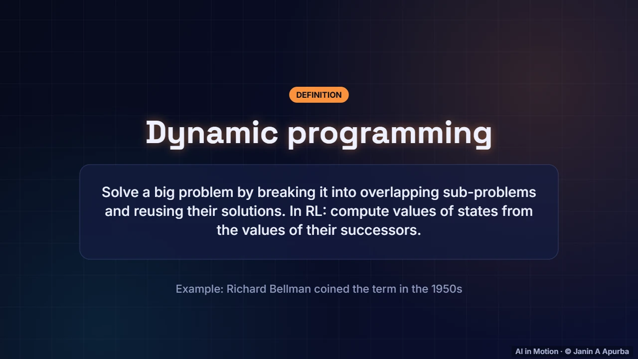
Dynamic programming, a term coined by Richard Bellman in the nineteen fifties, means solving a big problem by breaking it into smaller overlapping pieces and reusing their answers. In reinforcement learning, the value of each state is computed from the values of the states that follow it.
0:393. Planning with a model
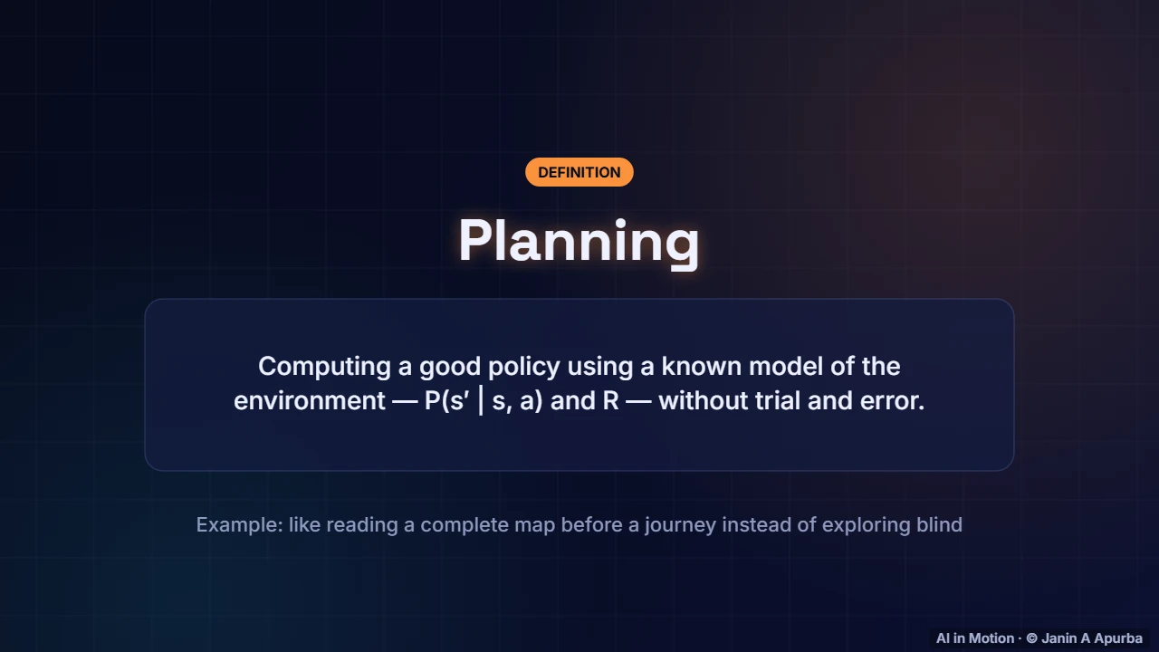
This is planning rather than learning. The agent has a complete model of the world: for every state and action, where it might end up and with what reward. It is like reading a detailed map before a journey instead of exploring blindly. Later lectures remove this assumption.
0:594. Our world
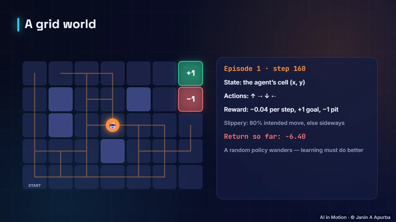
We return to our slippery grid world. Moves succeed eighty percent of the time and slip sideways otherwise, every step costs point zero four, the goal gives plus one and the pit minus one. Our task is to compute the value of every cell and the best action in every cell.
1:215. Bellman optimality
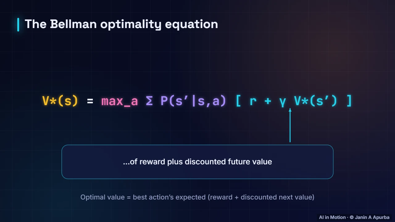
The key tool is the Bellman optimality equation. The best value of a state equals the maximum, over actions, of the expected reward plus discounted next value. The expectation averages over the slippery outcomes, and the maximum picks the best action. It is recursive: values depend on other values.
1:426. Expected updates
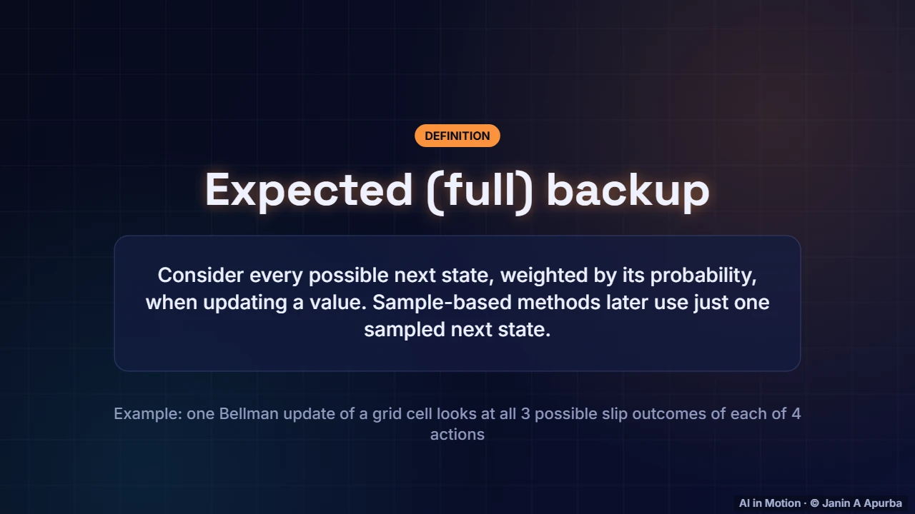
Dynamic programming uses expected updates. When it updates a cell, it considers every possible outcome of every action, weighted by its probability. In our grid that is three possible slip outcomes for each of four actions. Learning methods will later replace this full average with a single sampled outcome.
2:027. Worked example
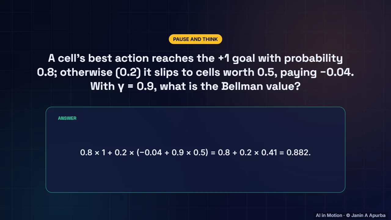
Let us compute one update by hand. The best action reaches the goal, worth plus one, with probability point eight. Otherwise it slips to cells worth point five and pays point zero four. The value is point eight, plus point two times minus point zero four plus point nine times point five, which is about point eight eight two.
2:268. Value iteration
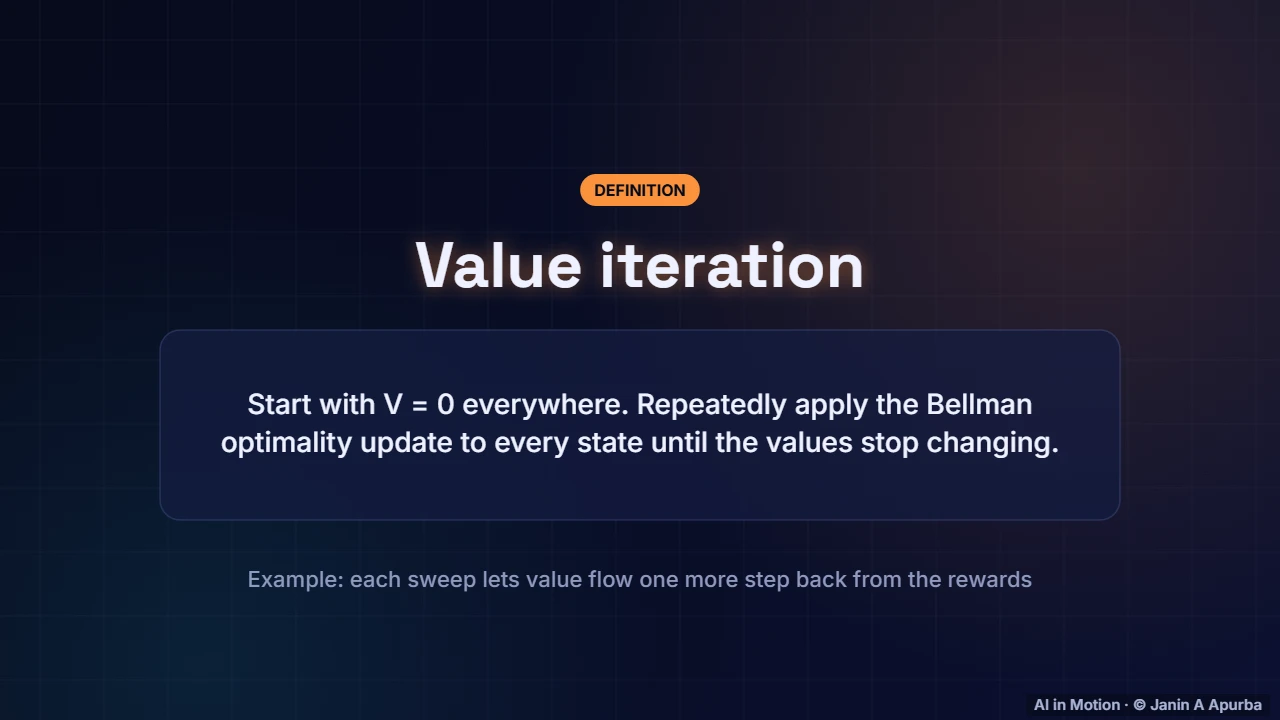
Value iteration turns that equation into an algorithm. Start with every value set to zero. Then sweep through all states, replacing each value with the right hand side of the Bellman equation computed from the current values. Repeat until nothing changes. Each sweep spreads information one step further.
2:479. Watching value iteration
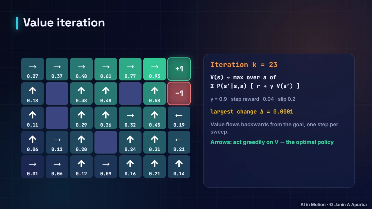
Watch it happen. After the first sweep, only cells next to the goal and pit know anything. Each sweep pushes value one step further back, like ripples spreading from the rewards. After twenty three sweeps the largest change drops below one ten thousandth, and the values have converged.
3:0710. Pause and think
Pause and think. After the very first sweep, why do only the cells right next to the goal or pit show strong values? Because each sweep looks just one step ahead, so only cells that can reach a terminal square in one move feel its reward. Information travels one step per sweep.
3:2911. The optimal policy
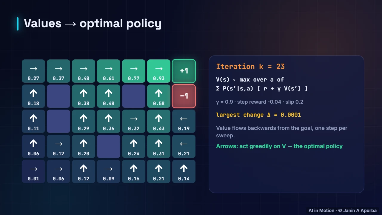
Once values have converged, the optimal policy falls out for free. In each cell, pick the action whose expected reward plus discounted next value is largest. The arrows lead around the walls towards the goal. Notice the cell just below the pit points left rather than up, because moving up would step straight into the pit.
3:5312. A non-slippery floor
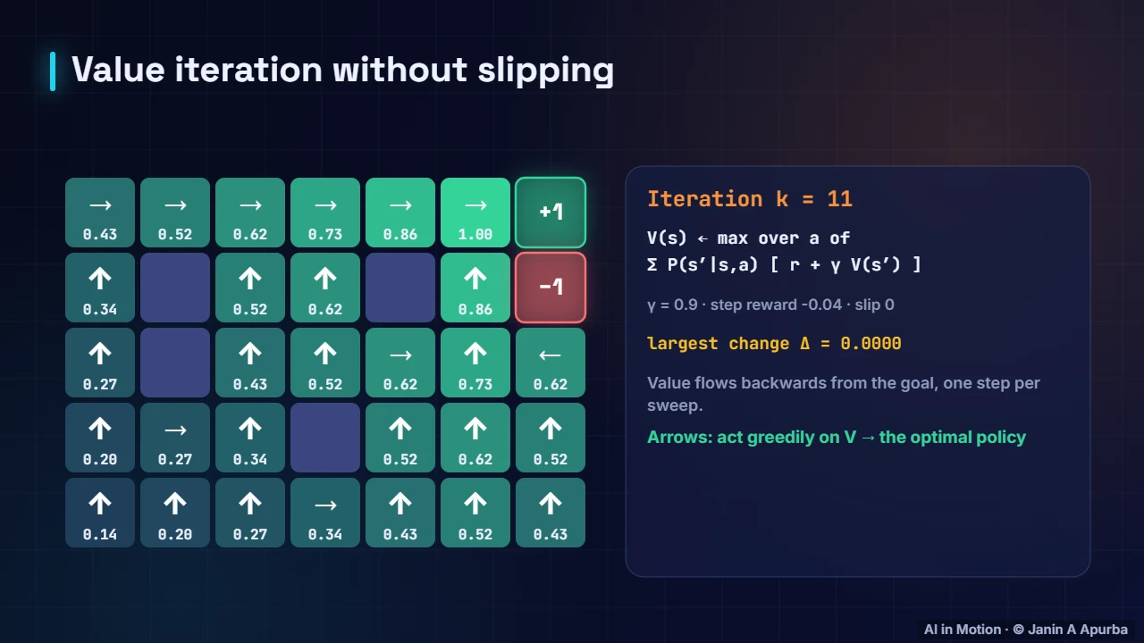
Now make the floor non slippery, so every move goes exactly where intended. Uncertainty was costing the agent a lot: the start cell is now worth about point one four instead of almost zero, and value iteration converges in eleven sweeps instead of twenty three, because outcomes are predictable.
4:1413. From values to action values
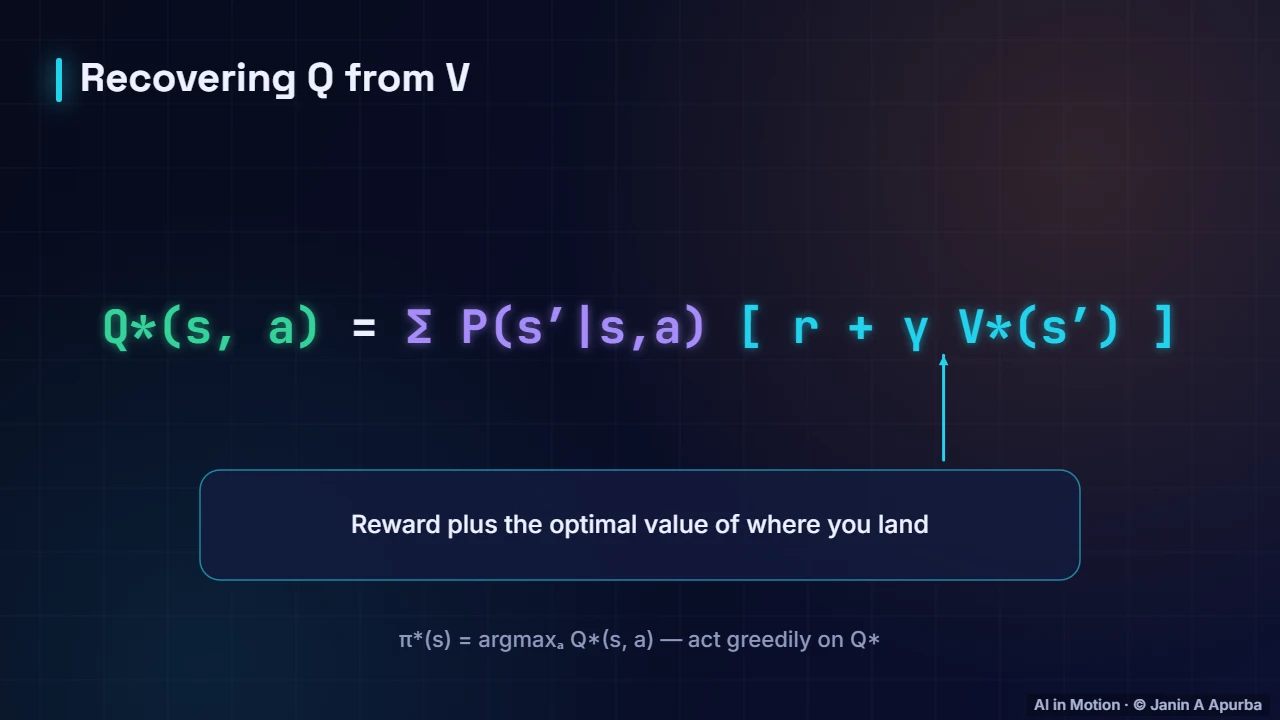
With a model, optimal action values follow directly from optimal state values: average reward plus discounted next value over the possible outcomes of each action. The optimal policy simply picks the action with the highest of these. Without a model, this step is impossible, which is why model free methods learn Q directly.
4:3614. Why it converges
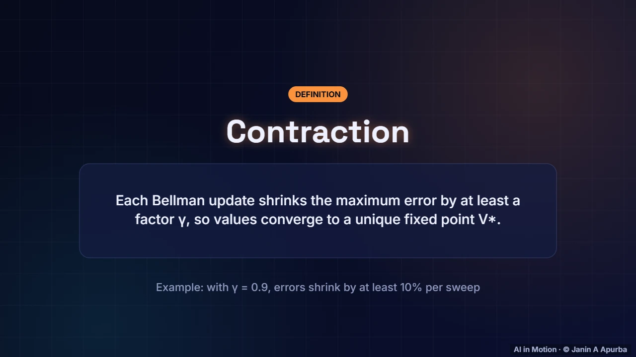
Why is convergence guaranteed? Each Bellman update is a contraction: it shrinks the largest error by at least a factor of gamma. With gamma of point nine, errors shrink by at least ten percent every sweep, so the values must converge to a unique fixed point, the optimal values.
4:5715. Policy evaluation
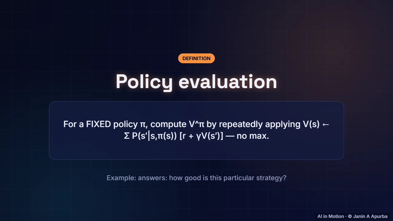
A related task is policy evaluation: given a fixed policy, how good is it? We apply the same kind of update but without the maximum, always using the policy’s own action. The result is the value of that policy in every state, which tells us exactly where the strategy is strong or weak.
5:1916. Policy improvement
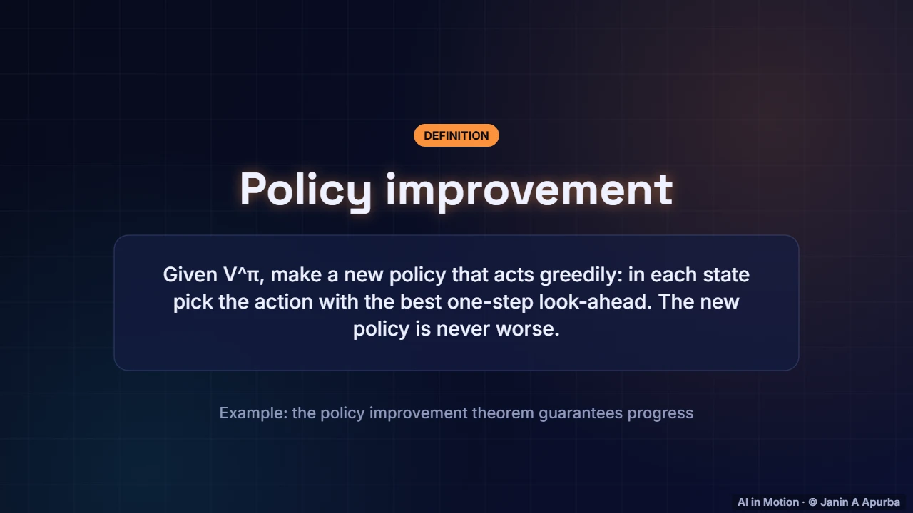
Once we know how good a policy is, we can improve it. In every state, look one step ahead with the current values, and switch to the best looking action. The policy improvement theorem guarantees the new policy is at least as good as the old one, and strictly better unless it was already optimal.
5:4217. Policy iteration
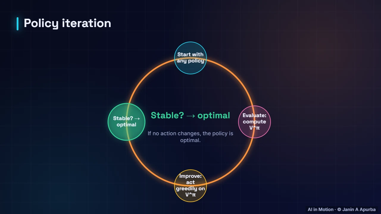
Alternating the two gives policy iteration. Start with any policy, even a silly one. Evaluate it, improve it, evaluate the new policy, improve again. Because each round is an improvement and there are finitely many policies, the process must stop, and when nothing changes the policy is optimal.
6:0318. Watching policy iteration
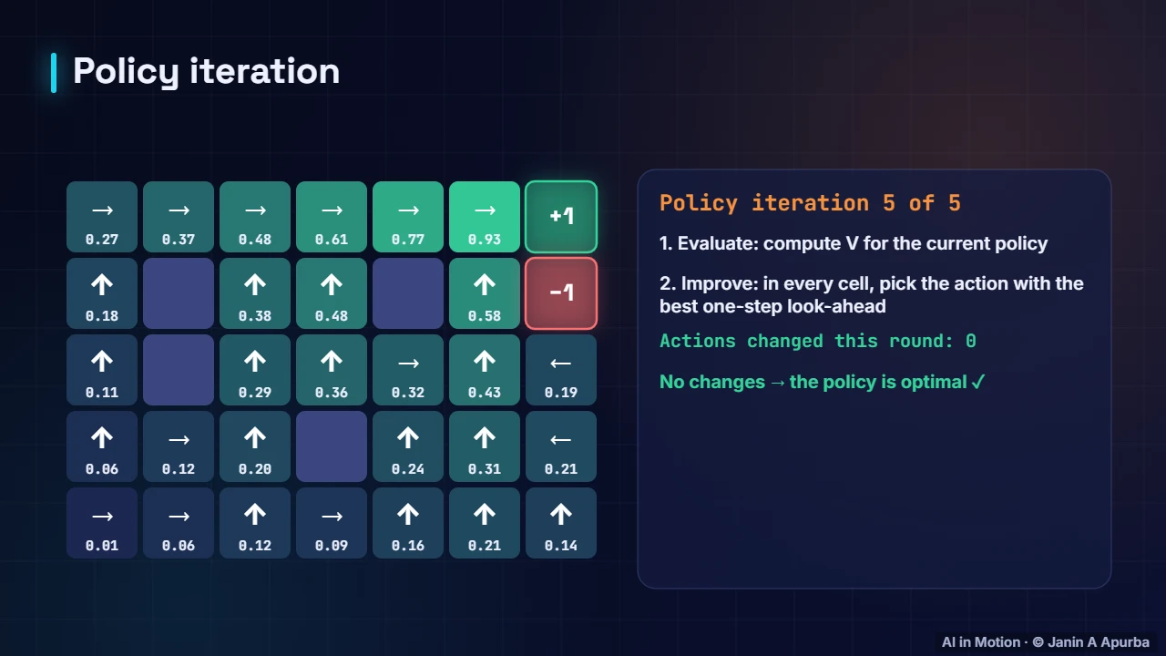
Here we start from the policy that always moves up. The first improvement changes twenty one of the cells. The next round changes ten, then one, then one, and in the fifth round nothing changes: the policy is optimal. Policy iteration typically needs only a handful of rounds.
6:2319. Value vs policy iteration
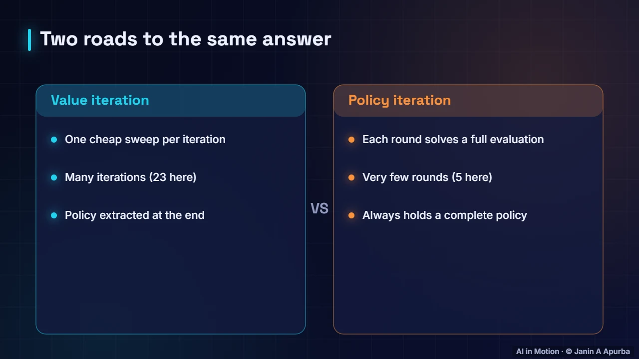
Both methods reach the same optimal policy. Value iteration uses many cheap sweeps, twenty three here. Policy iteration uses very few rounds, five here, but each round includes a complete policy evaluation. In practice, hybrids that do a few evaluation sweeps per improvement often work best.
6:4320. Pause and think
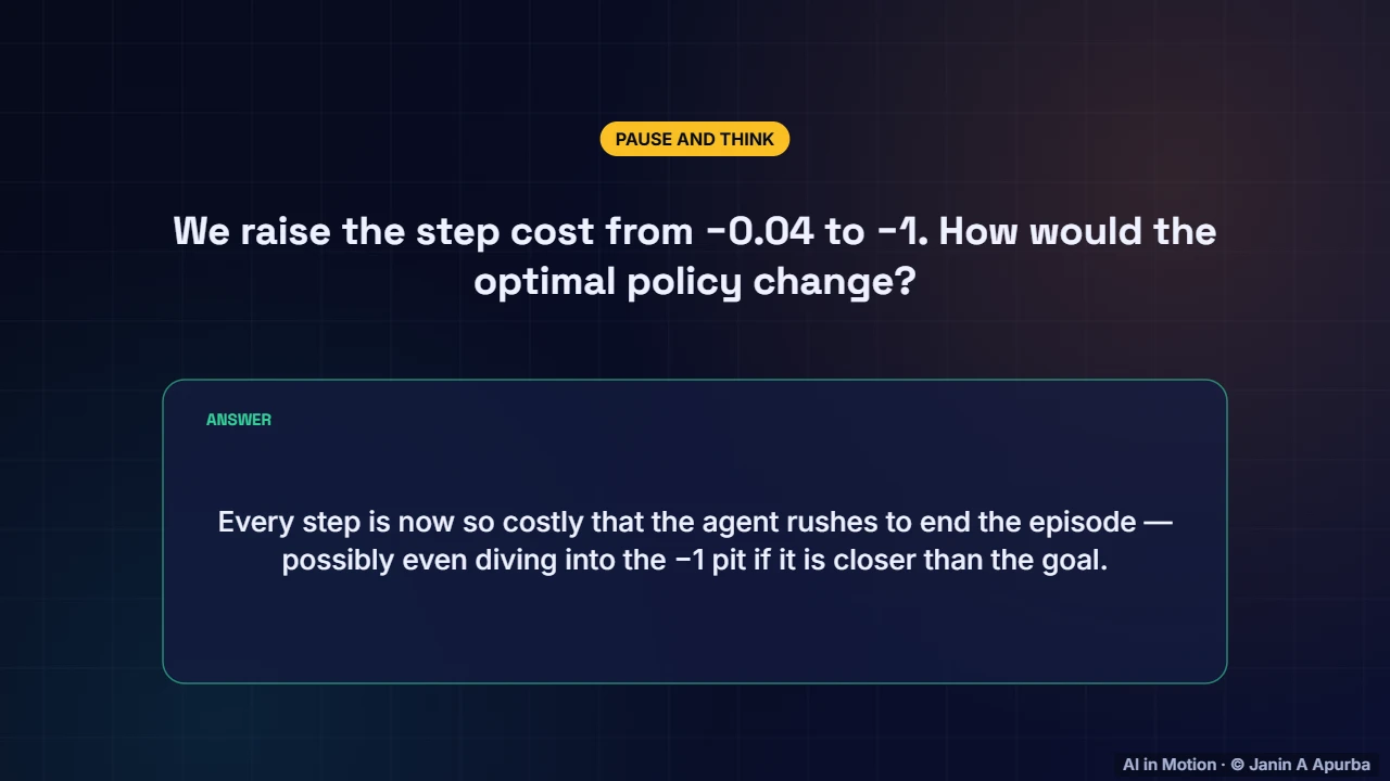
Pause and think. Suppose every step now costs minus one instead of minus point zero four. How would the optimal policy change? Each step is now so painful that the agent rushes to end the episode as quickly as possible, and from some cells even jumping into the minus one pit becomes the best choice.
7:0621. Reward design matters
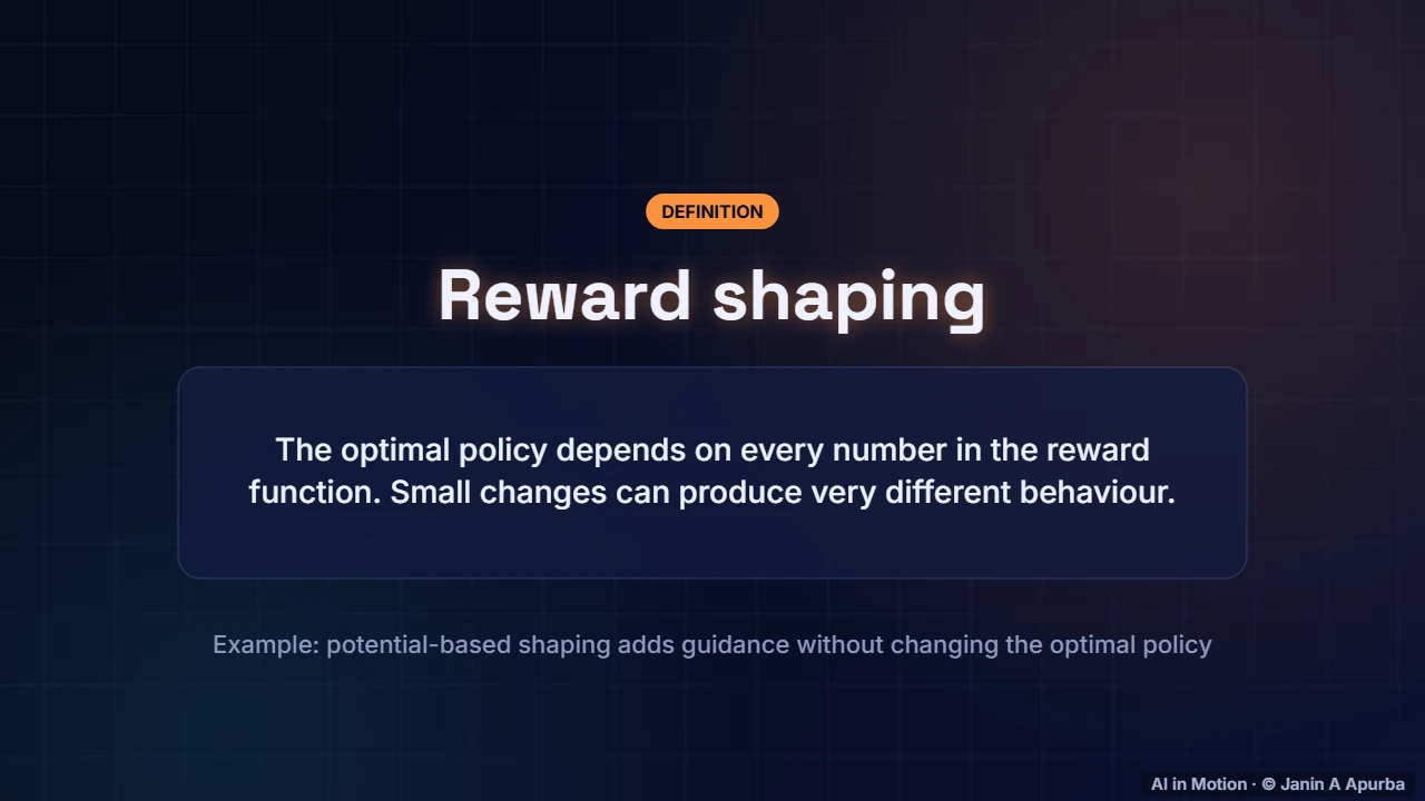
That example shows how sensitive behaviour is to the reward function. Every number matters. Reward shaping adds extra rewards to guide learning, but careless shaping can change what is optimal. A special form, potential based shaping, is proven to speed learning without changing the optimal policy.
7:2622. The role of gamma
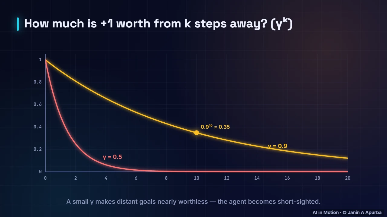
The discount factor also shapes the policy. With gamma of point nine, the goal reward seen from ten steps away is still worth about point three five. With gamma of one half it is worth less than a thousandth, so a far away goal becomes invisible and the agent becomes short sighted.
7:4823. Value iteration in code
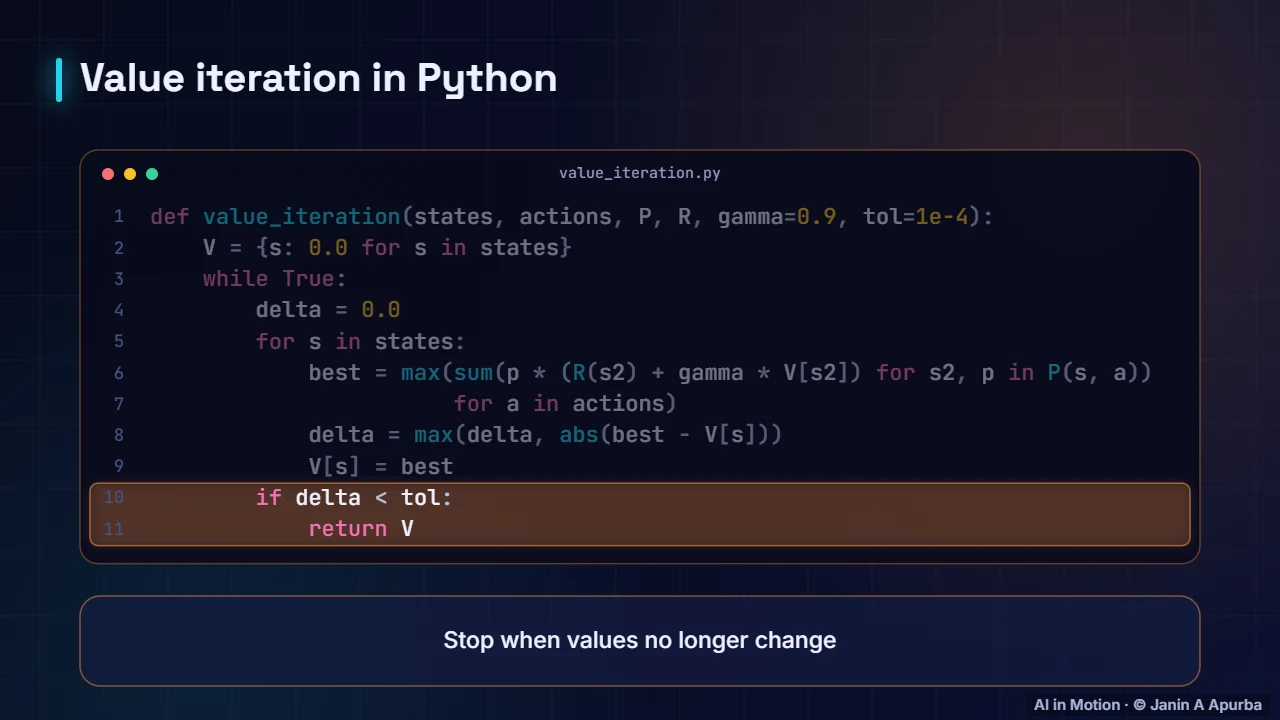
The whole algorithm fits in a dozen lines. Start with zero values. For every state, compute the best action’s expected reward plus discounted next value, record the largest change, and update. When the largest change falls below a small tolerance, stop. This is essentially what the animation computed.
8:0824. Computational cost
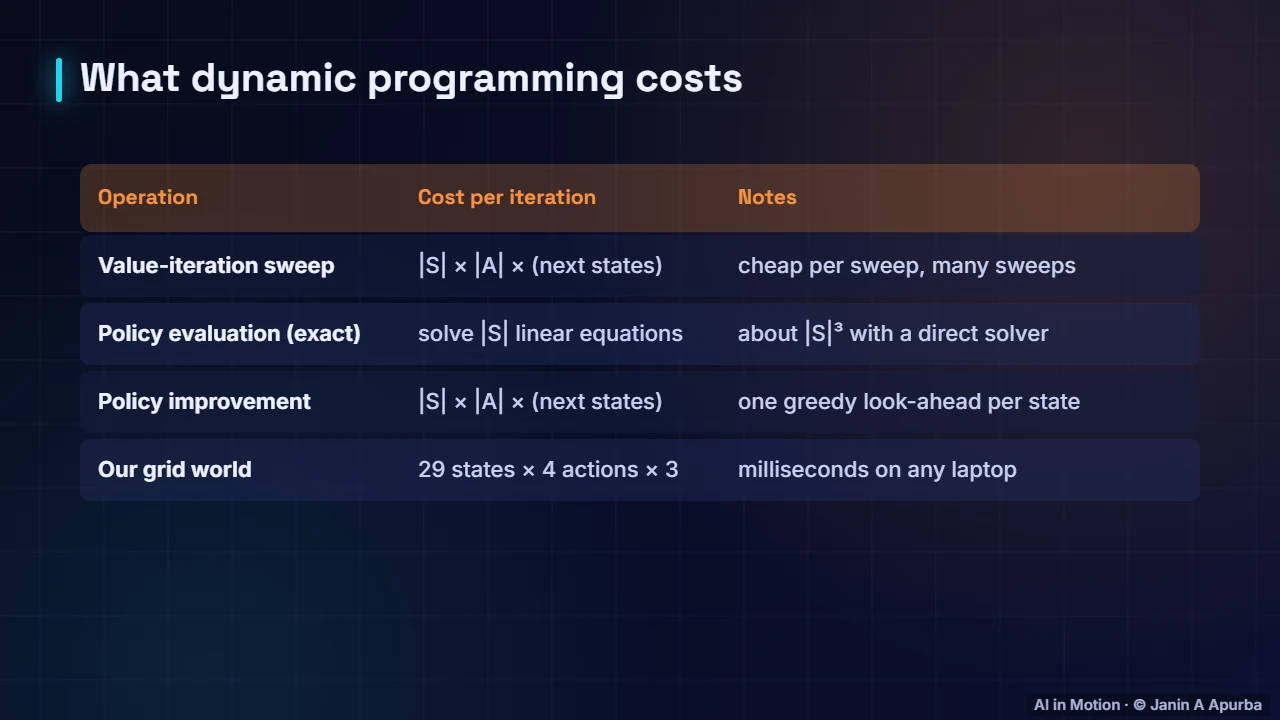
What does all this cost? Each value iteration sweep touches every state, every action and every possible next state. Exact policy evaluation solves a system of linear equations, roughly cubic in the number of states. For our little grid of twenty nine free cells, everything runs in milliseconds.
8:2925. Where DP is used
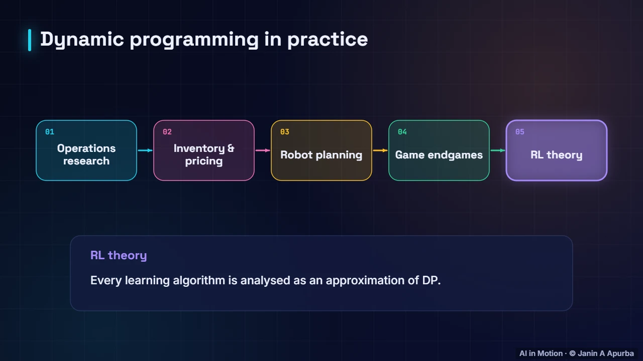
Dynamic programming remains useful whenever a good model exists and the state space is manageable: maintenance and queueing problems in operations research, inventory and pricing decisions, planning for robots on known maps, and exact endgame databases in chess. It is also the theoretical backbone that every learning method approximates.
8:4926. The curse of dimensionality
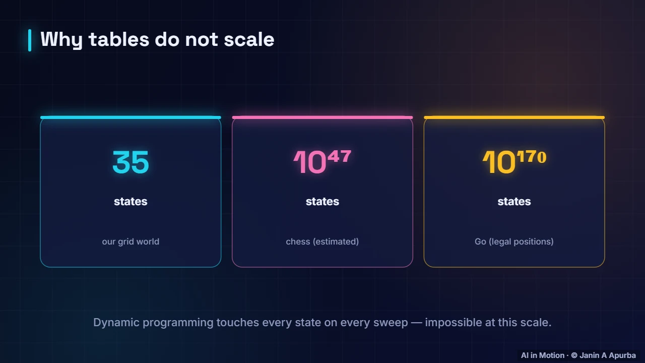
There is a catch. Dynamic programming touches every state on every sweep. Our grid has thirty five states, which is trivial. Chess has an estimated ten to the forty seven positions and Go about ten to the one hundred and seventy. No computer can sweep through those, so we need sampling and approximation.
9:1227. Asynchronous updates
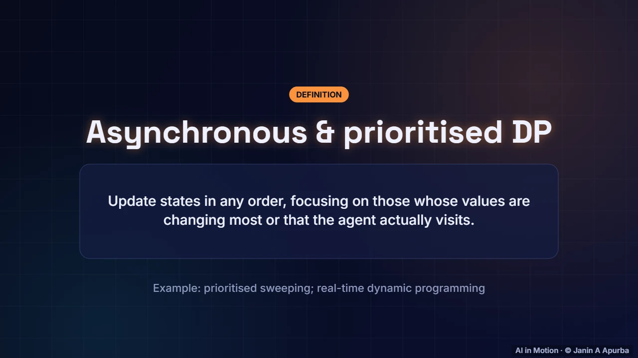
One response is to update states selectively rather than in full sweeps. Asynchronous dynamic programming updates states in any order, and prioritised sweeping focuses on states whose values are changing the most, or that the agent actually visits. This concentrates effort where it matters.
9:3128. Planning by search
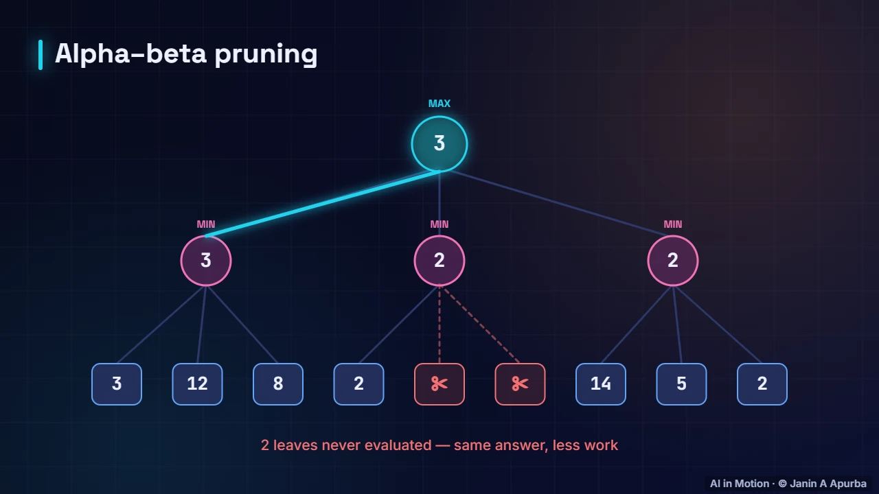
Another response is to plan only from the current state, looking ahead through a search tree. Game playing programs do this, and alpha beta pruning skips branches that cannot change the decision. AlphaZero combines this kind of look ahead with learned value functions, marrying planning and learning.
9:5129. Generalised policy iteration
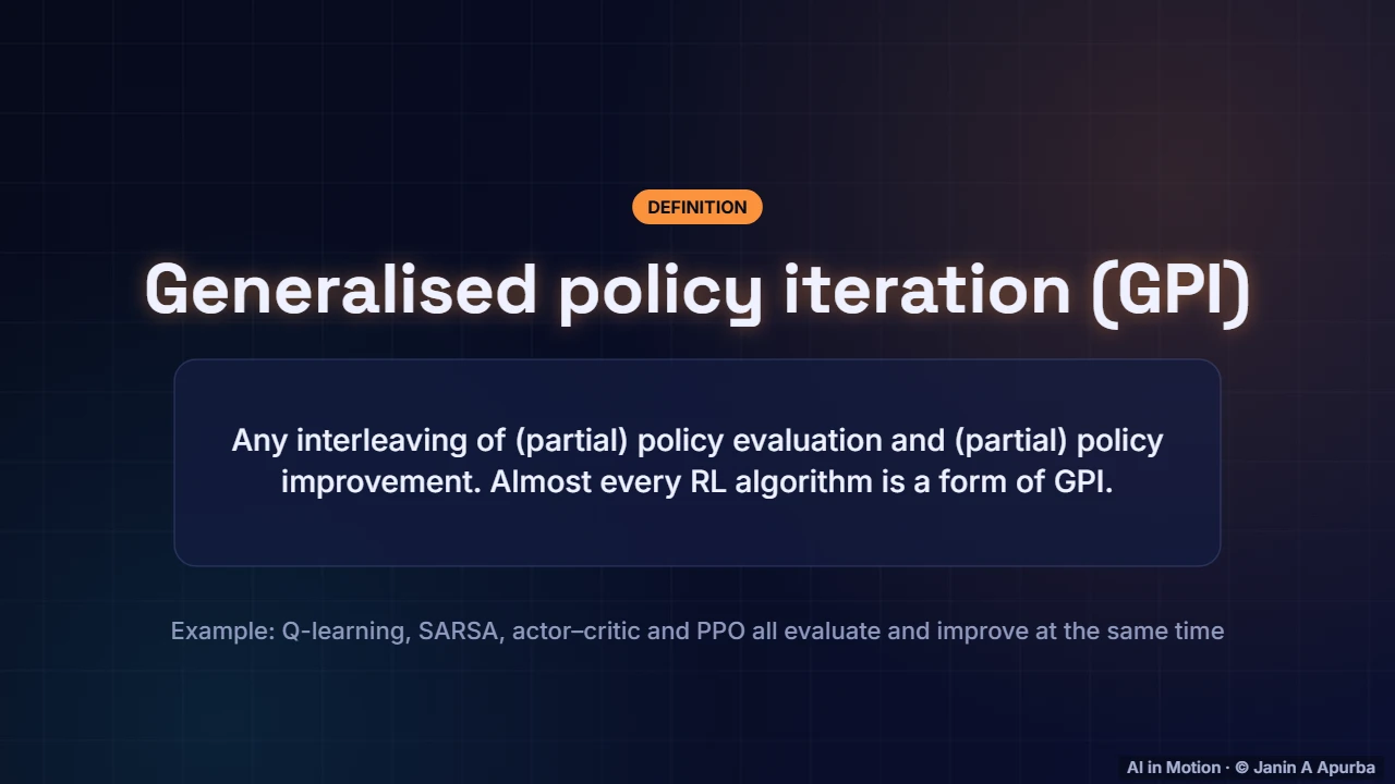
Here is the big idea to carry forward. Almost every reinforcement learning algorithm is a form of generalised policy iteration: some process that evaluates the current policy, interleaved with some process that improves it. Q learning, SARSA, actor critic methods and PPO all fit this pattern.
10:1030. Limitations
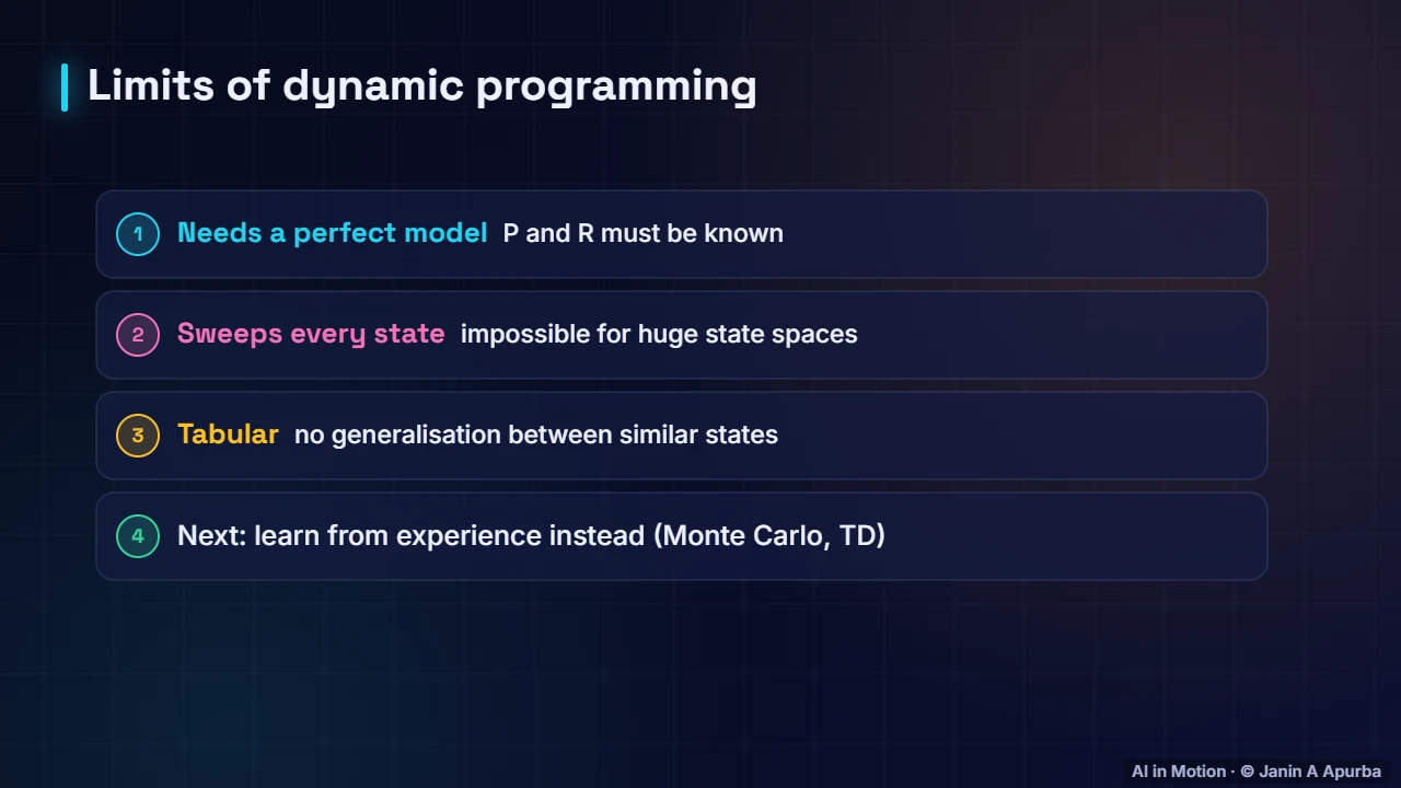
Dynamic programming has clear limits. It needs a perfect model of the environment, it sweeps every state, and it stores a separate number for each state with no generalisation. The next lecture removes the first limit, learning directly from experience with Monte Carlo and temporal difference methods.
10:3031. Pause and think
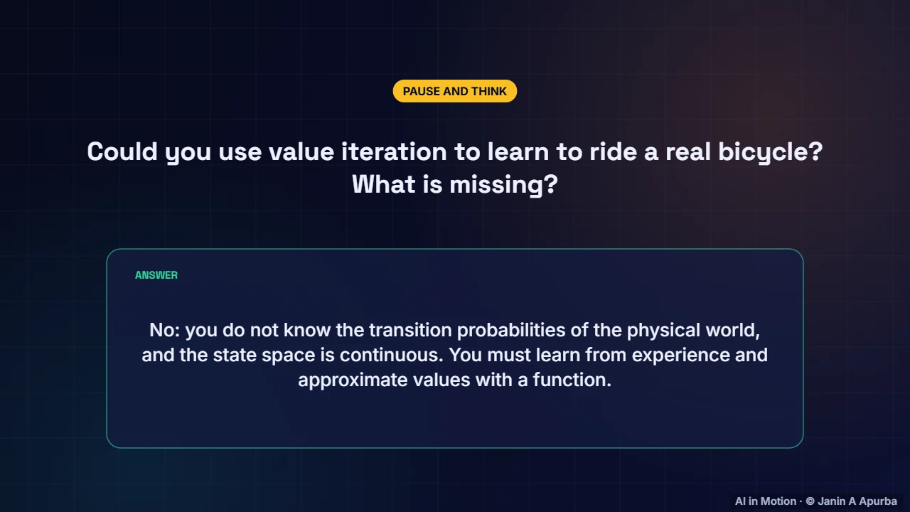
Pause and think. Could you use value iteration to learn to ride a real bicycle? Not directly. You do not know the transition probabilities of the physical world, and the state space is continuous. You must learn from experience and approximate values with a function, which is where the next lectures go.
10:5232. Recap
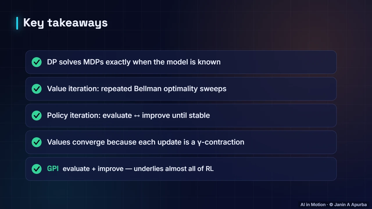
To recap. Dynamic programming solves MDPs exactly when the model is known. Value iteration applies Bellman optimality sweeps until values converge, and policy iteration alternates evaluation and improvement. Convergence follows from the contraction property, and the evaluate and improve pattern underlies almost all of reinforcement learning.
Key takeaways
- Dynamic programming plans with a known model: transition probabilities and rewards.
- Value iteration repeatedly applies V(s) ← max_a Σ P(s′|s,a)[r + γV(s′)] until convergence (23 sweeps in our grid).
- Policy iteration alternates policy evaluation and greedy improvement; it converged in 5 rounds here.
- The Bellman update is a γ-contraction, which guarantees convergence to V*.
- Rewards and γ strongly shape the optimal policy; reward design matters.
- Tabular DP does not scale to huge state spaces — motivating sampling and function approximation.
Check yourself
- What does value iteration need that Q-learning does not?
Show answer
A complete model of transitions and rewards — DP plans with a known model.
- In value iteration, how far does reward information travel per sweep?
Show answer
About one step — Each update looks one step ahead.
- Policy iteration alternates between…
Show answer
Policy evaluation and policy improvement — Evaluate, then improve greedily.
- Why does value iteration converge?
Show answer
Each Bellman update shrinks errors by at least a factor γ — The Bellman operator is a γ-contraction.
- What is generalised policy iteration?
Show answer
Any interleaving of policy evaluation and improvement — Most RL algorithms follow this pattern.
Go deeper
- Dynamic Programming: Policy Evaluation, Policy Iteration and Value Iteration · The AI Lecture Hall
- The Bellman Equations: Recursive Structure of Value · The AI Lecture Hall
- Markov Decision Processes: The Mathematical Framework of RL · The AI Lecture Hall
© 2026 Janin A Apurba, CSE, AUST · Advanced ICT Officer, CNRS-UNHCR. All rights reserved. Notes for the animated lecture at https://ai-in-motion.vercel.app/watch/dynamic-programming-value-and-policy-iteration.html