Convolutional Neural Networks: A Deep Dive — lecture notes
From pixels to predictions: why convolution, kernels and feature maps, stride, padding and channels, parameter counts, pooling, receptive fields, landmark architectures, residual connections, augmentation and transfer learning.
0:001. Introduction
Convolutional neural networks taught computers to see. They power photo search, medical imaging, self driving perception and the camera on your phone. In this deep dive we build a CNN from its smallest piece, the convolution, up to the architectures that won famous competitions.
0:182. Images are numbers
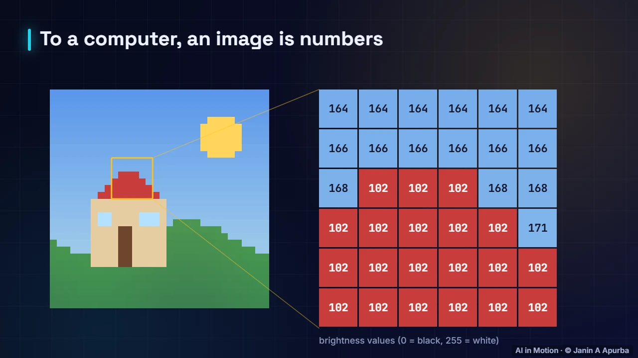
To a computer, an image is a grid of numbers. This small image is thirty two by thirty two pixels, and the yellow box zooms into a six by six patch. Each square is one pixel, and its number is its brightness, from zero for black to two hundred and fifty five for white.
0:413. Colour channels
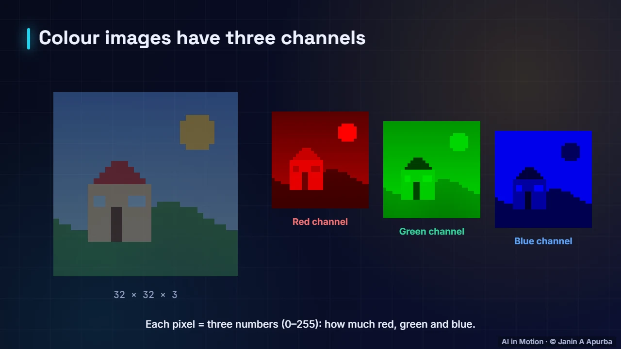
Colour images store three numbers per pixel: how much red, green and blue light to mix. So a colour image is really three grids stacked together, called channels. A thirty two by thirty two colour image holds thirty two times thirty two times three, which is three thousand and seventy two numbers.
1:034. Pause and think
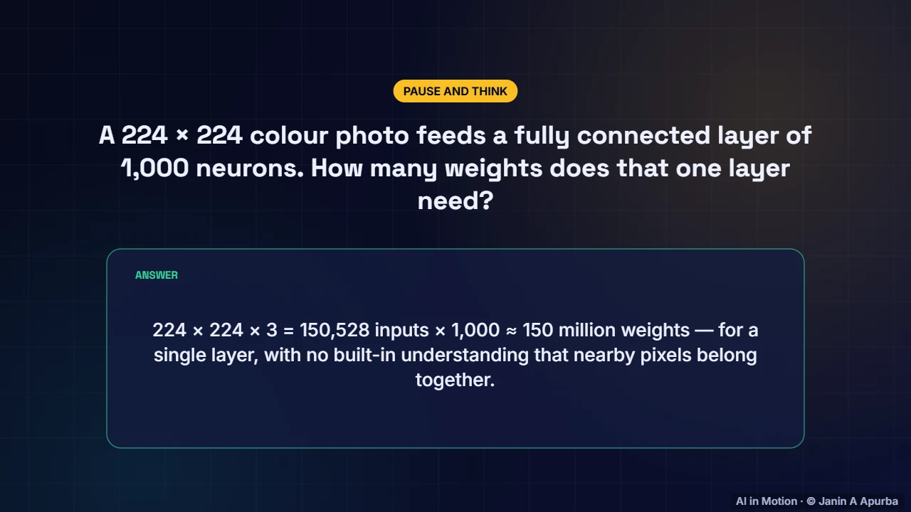
Pause and think. A standard two hundred and twenty four pixel colour photo feeds a fully connected layer of one thousand neurons. How many weights is that? About one hundred and fifty thousand inputs times a thousand: roughly one hundred and fifty million weights, for just one layer.
1:245. Why convolution?
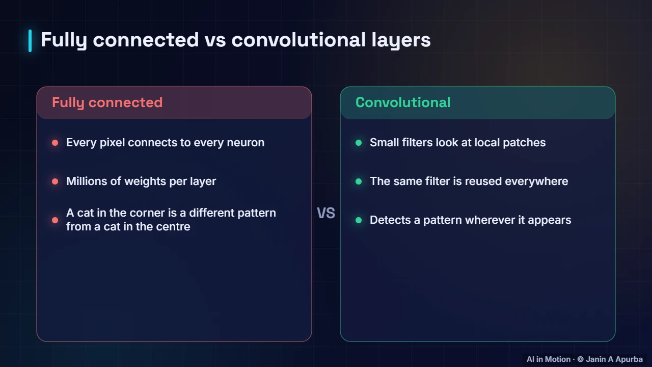
Convolution solves this. Instead of connecting every pixel to every neuron, a small filter looks at one local patch at a time, and the same filter slides across the whole image. That shares weights, cutting parameters enormously, and lets the network recognise a pattern wherever it appears.
1:446. The convolution operation
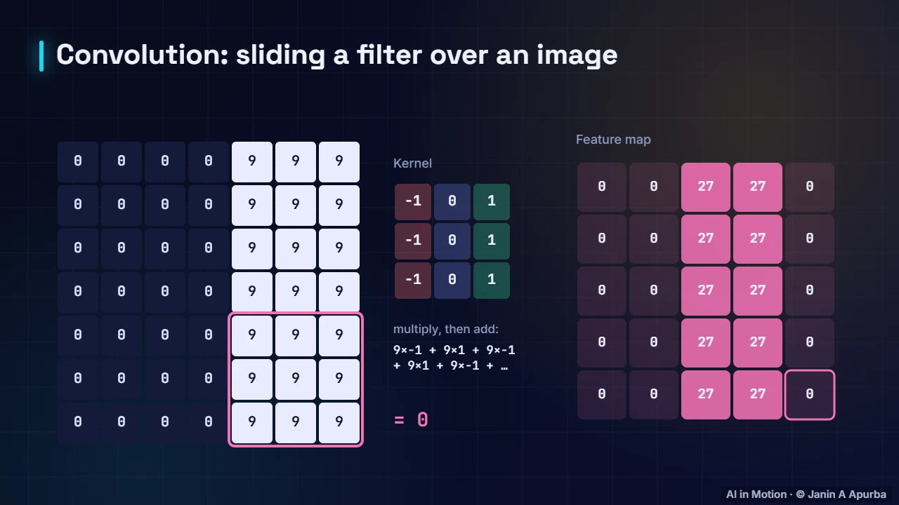
Here is convolution in action. The image is dark on the left and bright on the right. The kernel is a three by three grid of numbers. Place it over a patch, multiply each pair of numbers, add them up, then slide one step and repeat. The feature map lights up with twenty sevens exactly where dark meets bright: an edge.
2:087. The formula
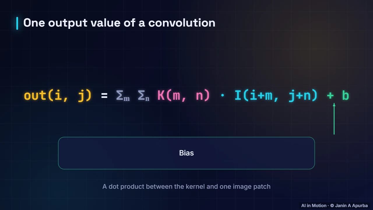
Each output value is a dot product between the kernel and one image patch, plus a bias. Sliding the kernel over every position produces a whole feature map, showing where in the image the kernel’s pattern appears. Strictly this is cross correlation, but deep learning calls it convolution.
2:288. Blurring
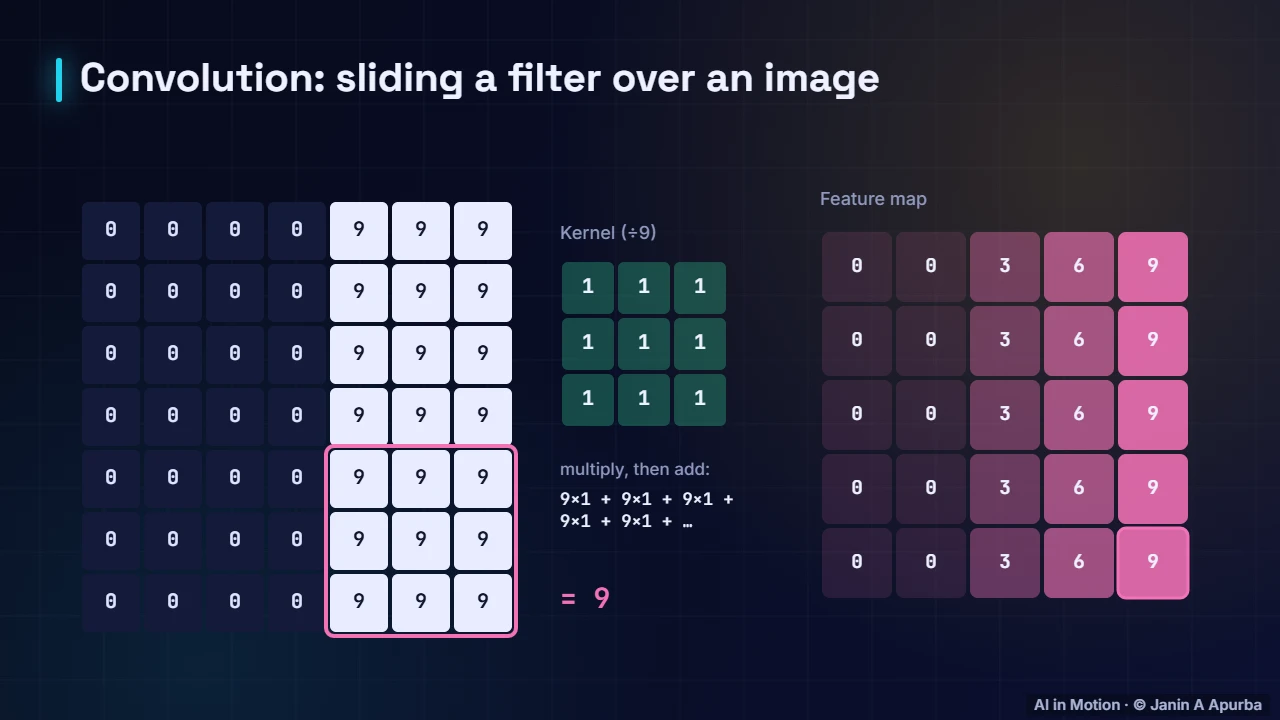
Different kernels detect different things. A blur kernel has every weight equal to one ninth, so each output is the average of its neighbourhood. The sharp jump from zero to nine becomes a gentle ramp: zero, three, six, nine.
2:459. Sharpening
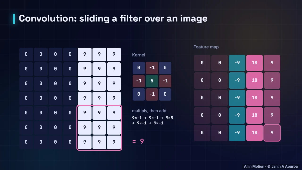
A sharpen kernel does the opposite. It boosts the centre pixel and subtracts its neighbours, exaggerating differences. Around the edge we get minus nine on the dark side and eighteen on the bright side, making the edge stand out even more.
3:0310. Classic edge detection
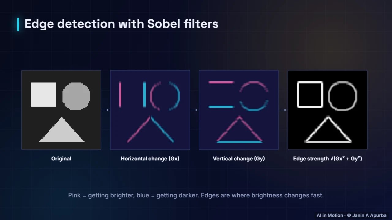
Before deep learning, engineers designed kernels by hand. The Sobel filters detect horizontal and vertical changes in brightness, and combining them gives edge strength in every direction. Classic computer vision pipelines were built from carefully designed filters like these.
3:1911. Learned filters
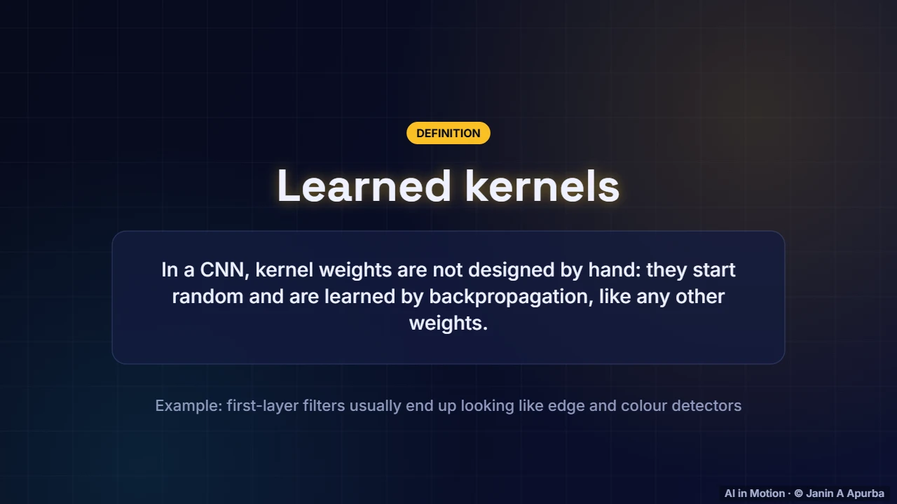
The breakthrough of CNNs is that kernels are learned, not designed. They start random and are adjusted by backpropagation, like any other weights. Remarkably, the filters learned in the first layer usually end up resembling edge and colour detectors, rediscovering what engineers once designed by hand.
3:3912. Output size
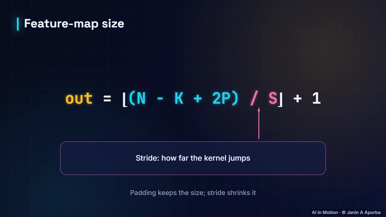
Two settings control the output size. Padding adds a border of zeros so the kernel can sit on edge pixels, and stride is how far the kernel jumps each time. The output size is the input size minus the kernel size plus twice the padding, divided by the stride, plus one.
4:0113. Compute it
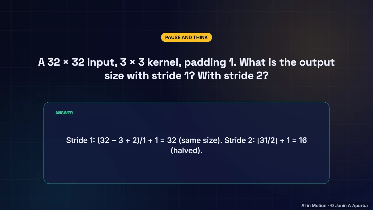
Let us compute. A thirty two by thirty two input, a three by three kernel and padding of one. With stride one, the output is thirty two minus three plus two, plus one: thirty two, the same size. With stride two, it is halved to sixteen.
4:2014. Channels and filters
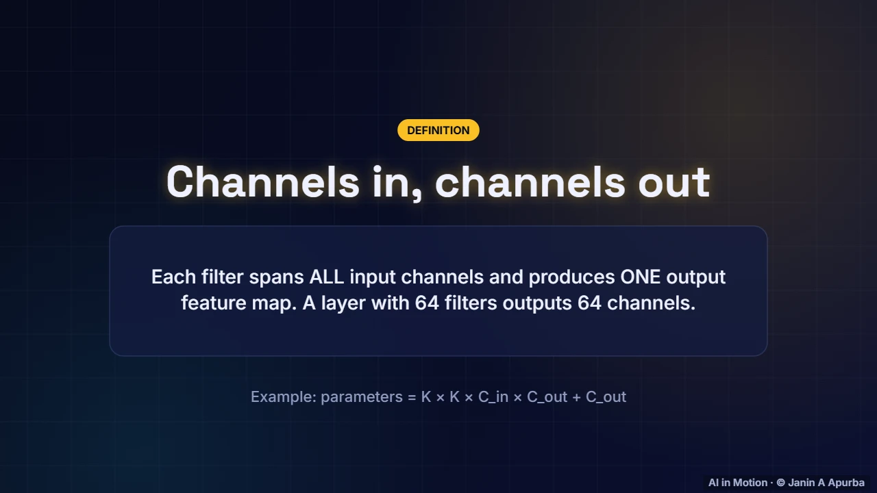
Real layers work with many channels. Each filter extends through all the input channels and produces one output feature map, so a layer with sixty four filters outputs sixty four channels. The parameter count is kernel height times width times input channels times output channels, plus one bias per filter.
4:4215. Pause and think
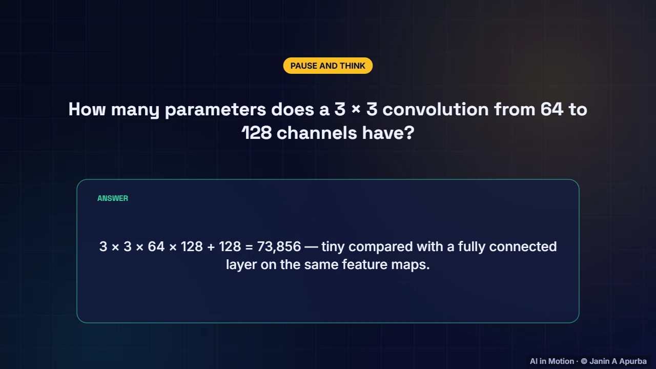
Pause and think. How many parameters does a three by three convolution from sixty four to one hundred and twenty eight channels have? Three times three times sixty four times one hundred and twenty eight, plus one hundred and twenty eight biases: seventy three thousand, eight hundred and fifty six.
5:0316. Max pooling
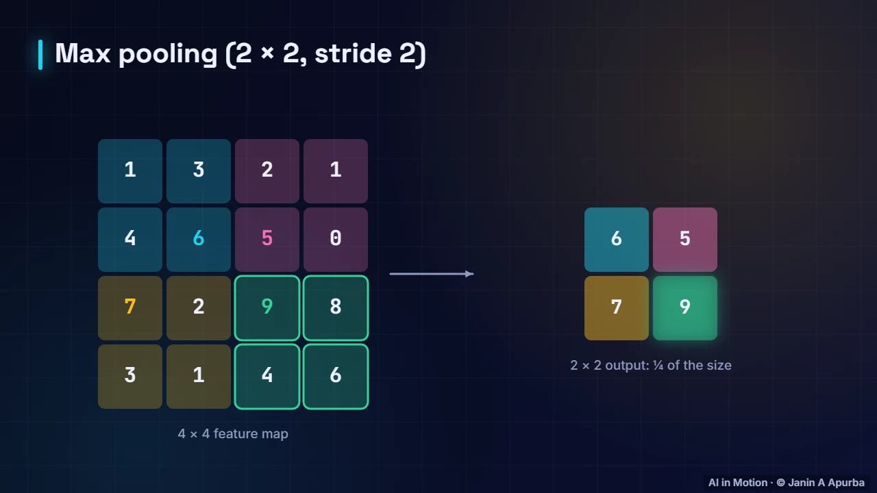
Pooling layers shrink feature maps. Max pooling slides a two by two window with a stride of two and keeps only the largest value in each window: six, five, seven and nine. The four by four map becomes two by two, a quarter of the size, keeping the strongest signals.
5:2417. Average pooling
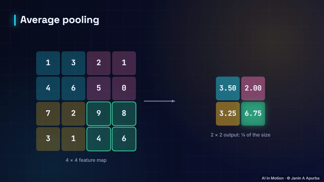
Average pooling keeps the mean of each window instead: three and a half, two, three and a quarter, and six and three quarters. It is smoother. A global version, averaging a whole feature map to one number, is common at the end of modern networks, replacing large fully connected layers.
5:4518. A complete CNN
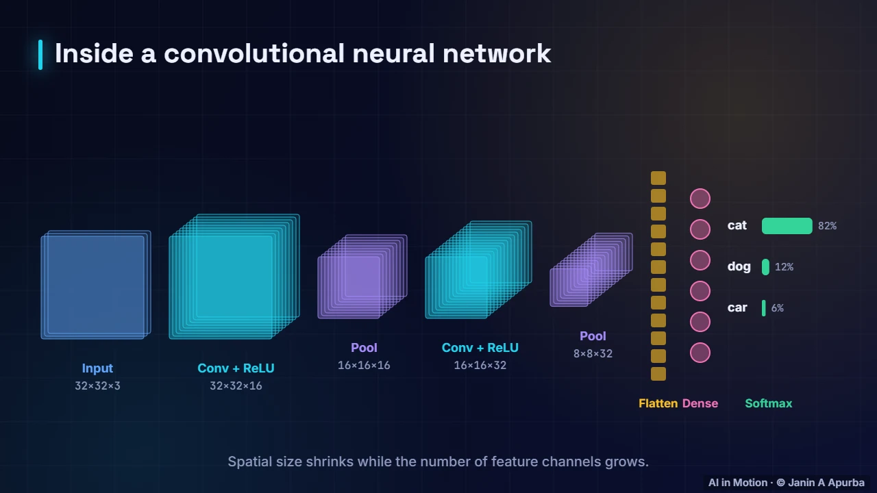
Now follow the data through a complete network. A thirty two by thirty two colour image enters. A convolution layer applies sixteen learned filters, and pooling halves the size. Another convolution makes thirty two maps and pooling shrinks again. Space shrinks while channels grow, and a final dense layer outputs class probabilities.
6:0719. Receptive field
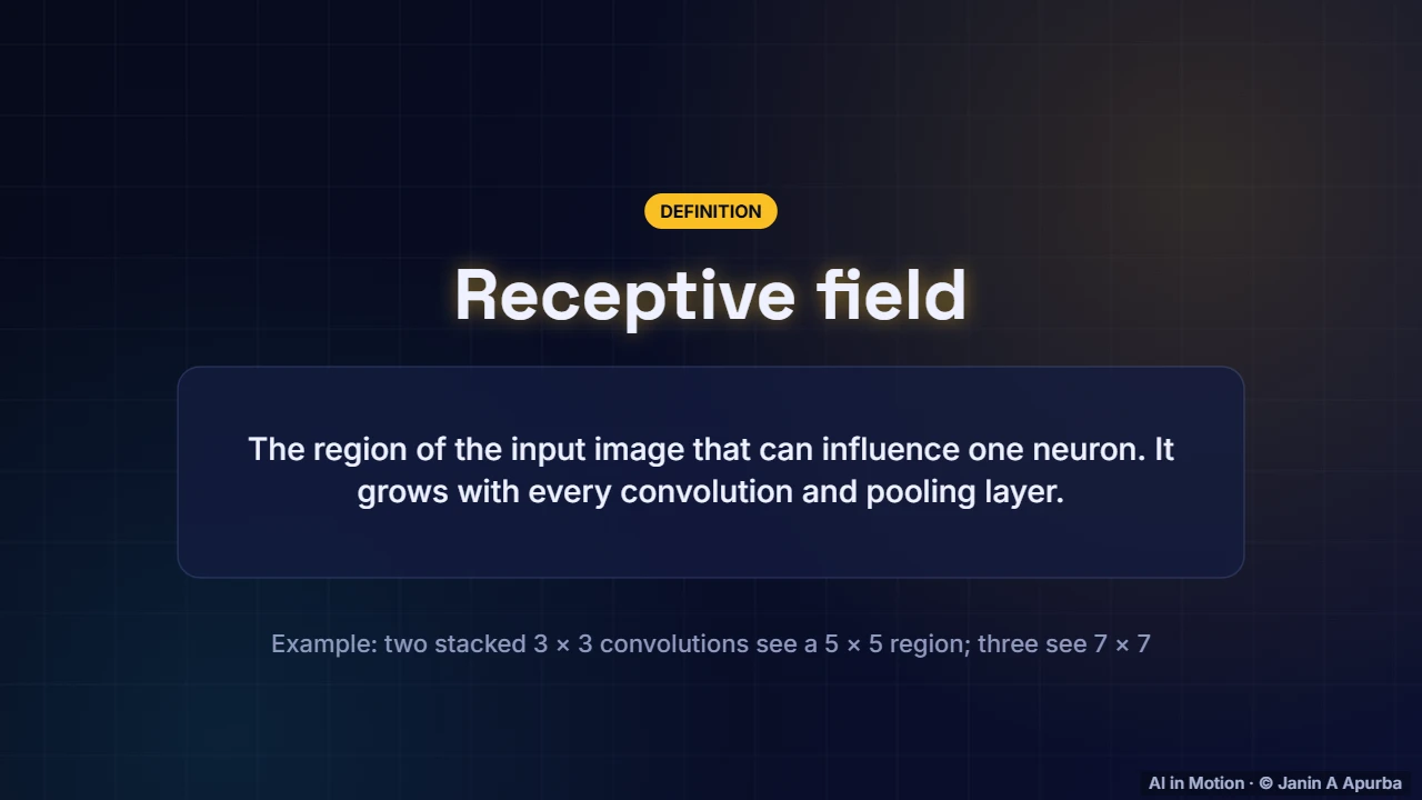
Each neuron’s receptive field is the part of the input image that can influence it. It grows with every layer: two stacked three by three convolutions see a five by five region, three see seven by seven, and pooling enlarges it faster. Deep neurons can therefore respond to whole objects.
6:2820. The feature hierarchy
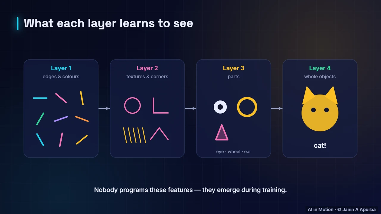
What does each layer learn? The first layers detect edges and colours. The next combine them into textures and corners. Deeper layers respond to parts like eyes and wheels, and the deepest to whole objects. Nobody programs these features. They emerge from training on labelled images.
6:4821. Classification
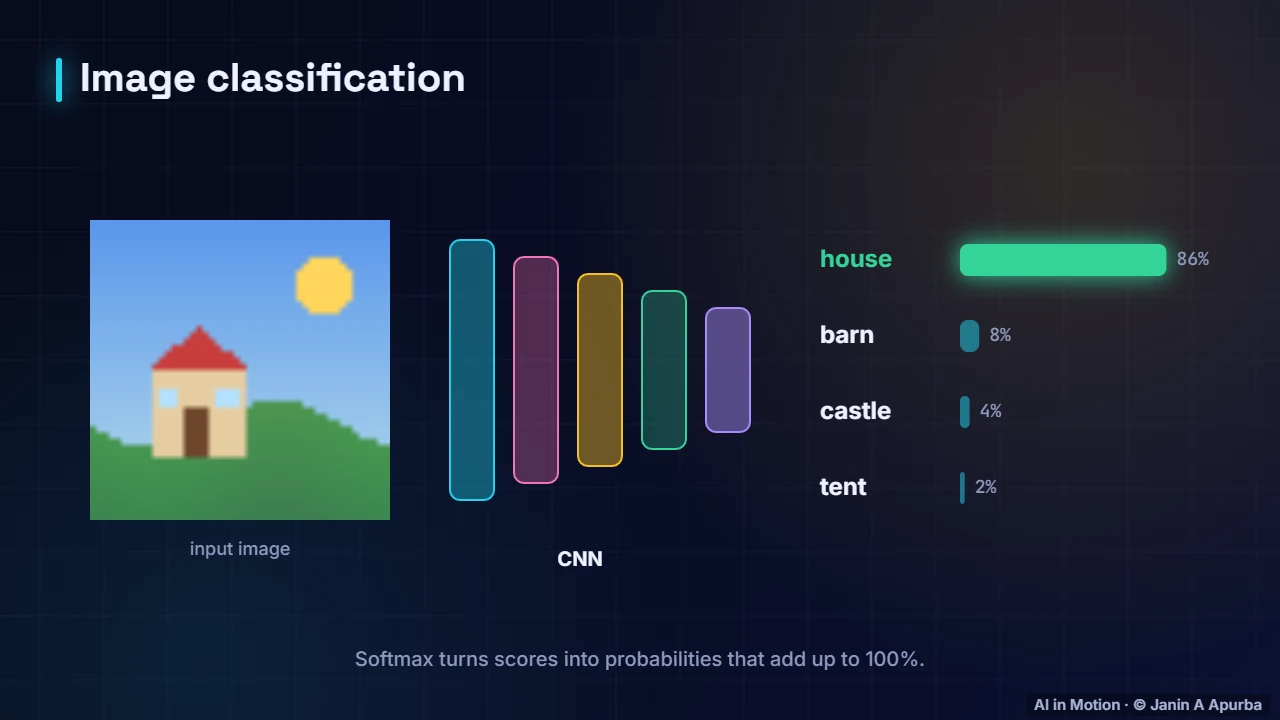
At the end, the network outputs a score for every class, and softmax turns the scores into probabilities that add up to one hundred percent. Here it is eighty six percent confident that this image shows a house. The loss compares this distribution with the true label.
7:0822. Landmark architectures
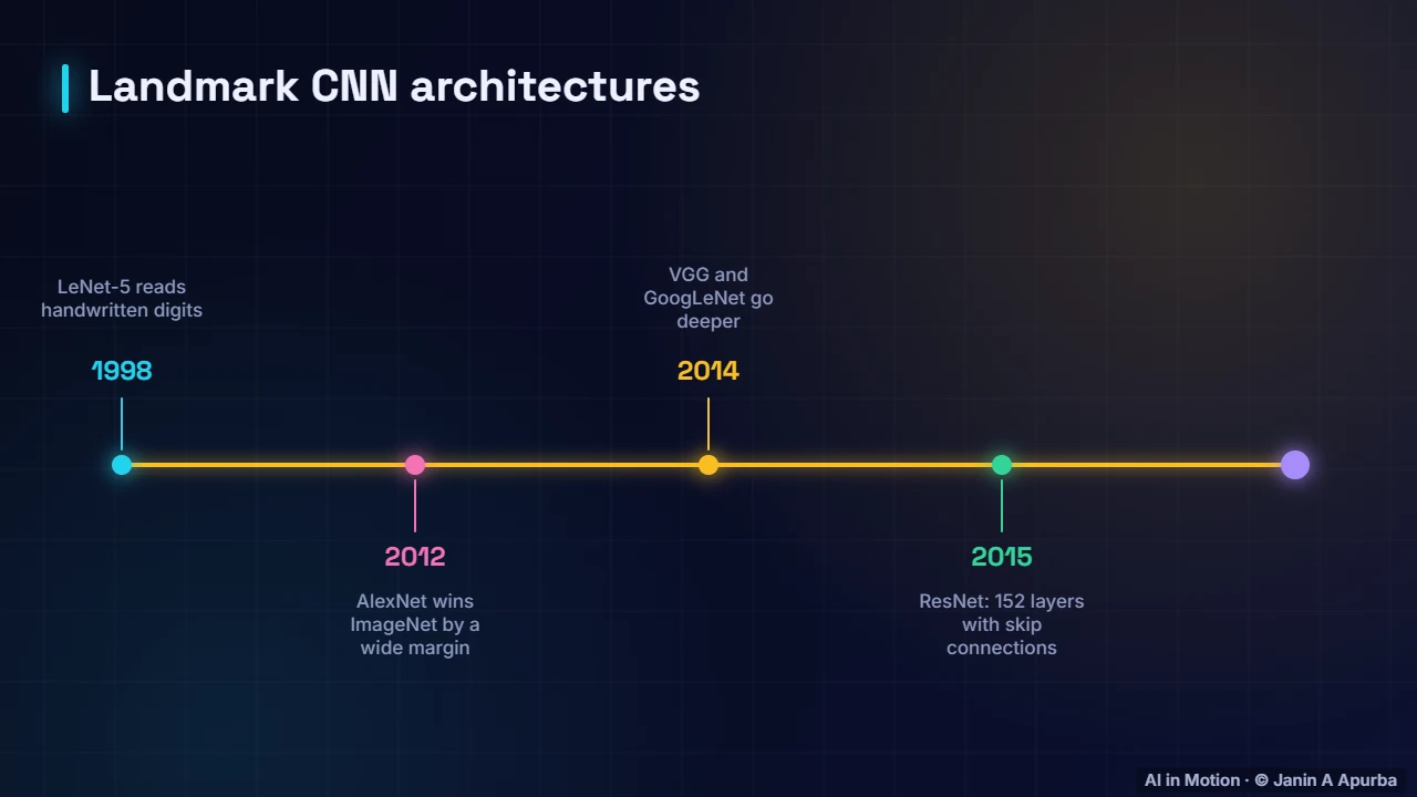
CNNs have a rich history. LeNet five read handwritten digits in 1998. AlexNet won the ImageNet competition in 2012 by a wide margin, launching the deep learning era. VGG and GoogLeNet went deeper in 2014, ResNet reached one hundred and fifty two layers in 2015, and EfficientNet scaled networks systematically in 2019.
7:3023. Why ResNet mattered
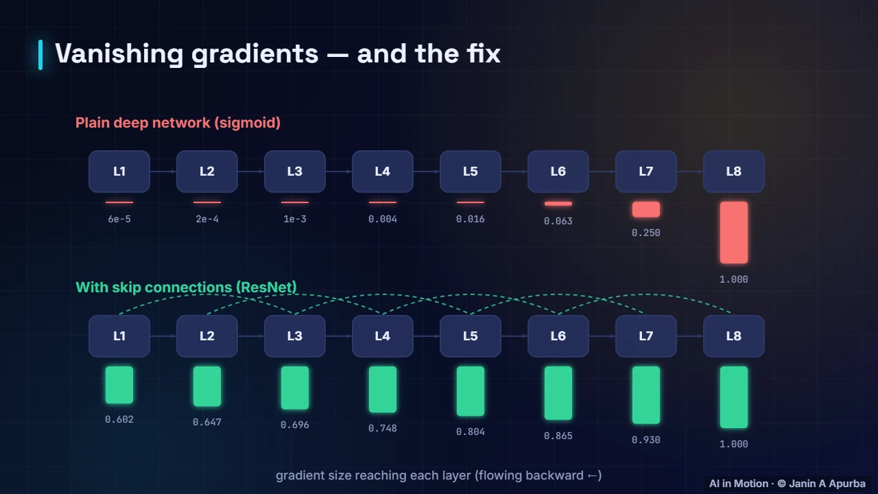
Why could ResNet go so deep? Each residual block adds its input to its output, giving gradients a direct highway back to early layers. Without skip connections, gradients fade through many layers. With them, networks with over a hundred layers train reliably and outperform shallower ones.
7:5024. Batch normalisation

Most CNNs also use batch normalisation. After a convolution, each channel’s activations are normalised using the mini batch’s mean and variance, then scaled and shifted by learned parameters. The classic building block is convolution, then batch norm, then ReLU. It allows higher learning rates and deeper networks.
8:1025. Data augmentation
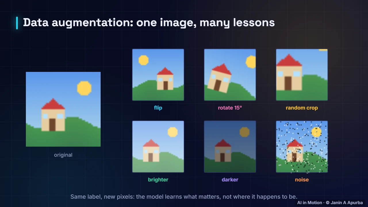
Vision models need lots of varied data, and augmentation multiplies what we have. Flip an image, rotate it slightly, crop a random region, change the brightness or add noise. The label stays the same, so the network learns that these changes do not matter, and it overfits far less.
8:3126. Transfer learning
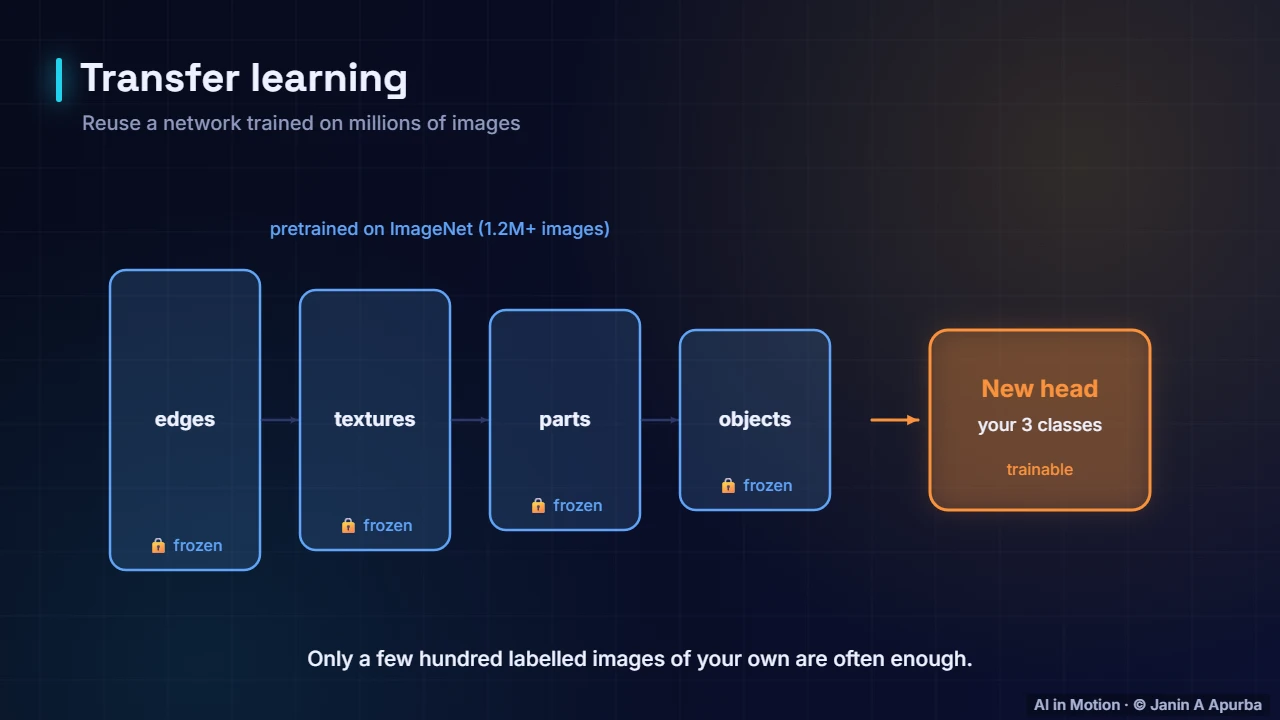
You rarely train a vision model from scratch. Take a network pre trained on ImageNet, with over a million images. Its layers already detect edges, textures, parts and objects. Freeze them, remove the original classifier, and add a new head for your own classes. Only the head is trained.
8:5127. Fine-tuning
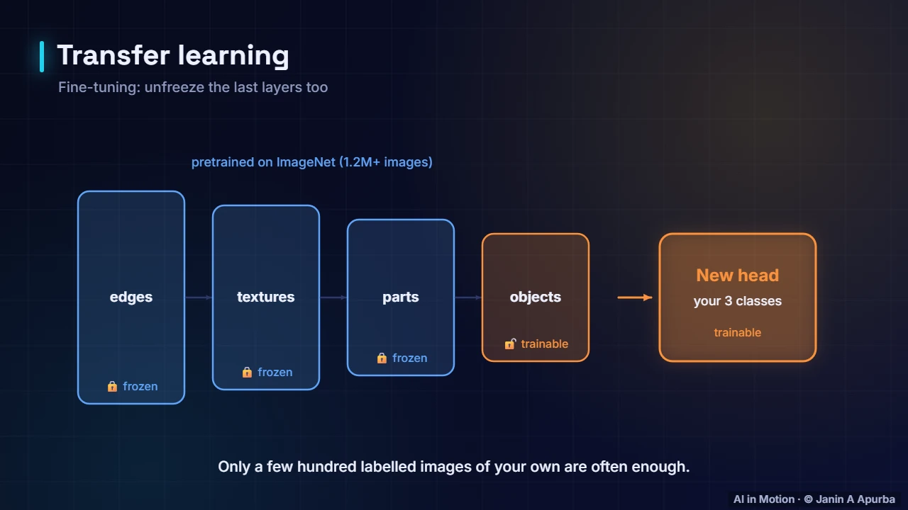
With a bit more data, unfreeze the last block as well and fine tune it with a small learning rate. Early layers stay frozen, because edges and textures are useful for almost any task. This approach reaches strong accuracy with just hundreds of images per class.
9:1128. A CNN in code
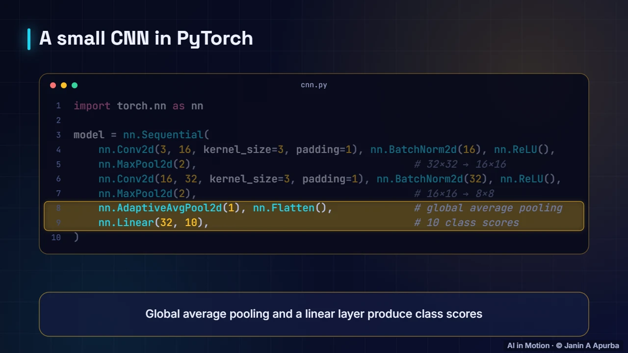
Here is a small CNN in PyTorch. Two blocks of convolution, batch norm and ReLU, each followed by max pooling, take a thirty two pixel image down to eight by eight with thirty two channels. Global average pooling and a linear layer then produce scores for ten classes.
9:3129. Beyond CNNs
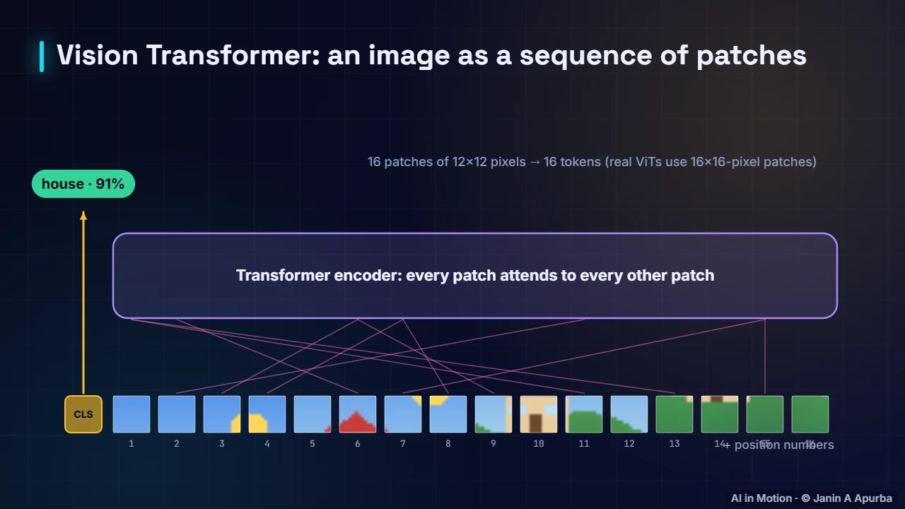
Vision transformers offer an alternative. The image is cut into patches, each turned into an embedding like a word, and a transformer lets every patch attend to every other patch. With enough data they match or beat CNNs, and many modern systems combine ideas from both.
9:5130. CNNs vs vision transformers
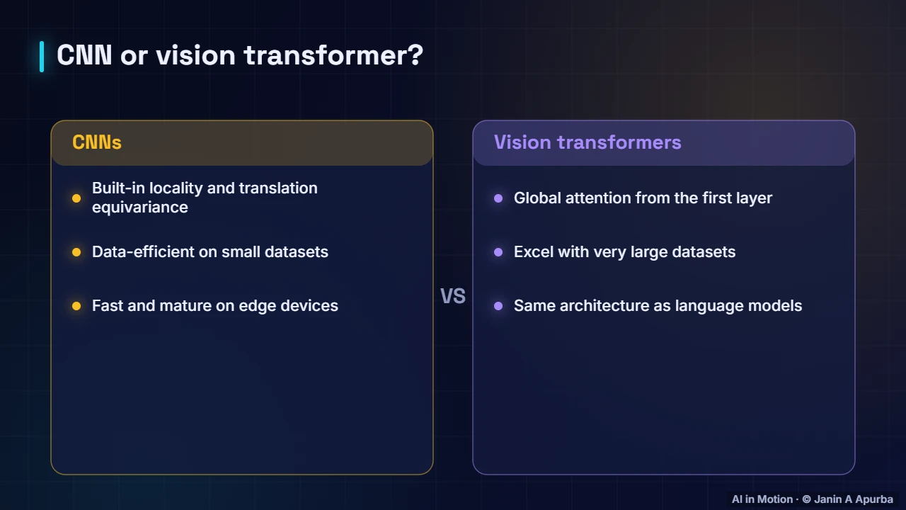
Which should you choose? CNNs have useful built in assumptions about locality, so they learn well from smaller datasets and run efficiently on phones. Vision transformers apply global attention from the start, shine with very large datasets, and share their architecture with language models, which simplifies multimodal systems.
10:1131. Practical tips
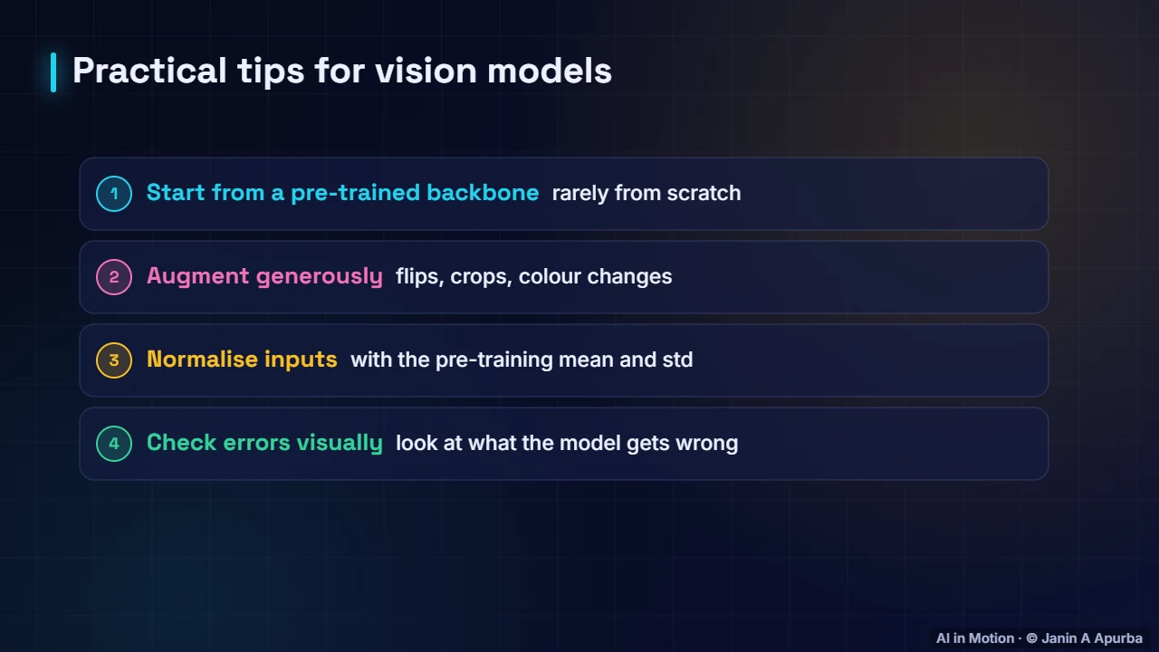
Some practical tips. Start from a pre trained backbone. Augment generously. Normalise inputs with the same mean and standard deviation used in pre training. And look at the images the model gets wrong: visual error analysis often reveals labelling mistakes, missing classes or misleading shortcuts.
10:3132. Recap
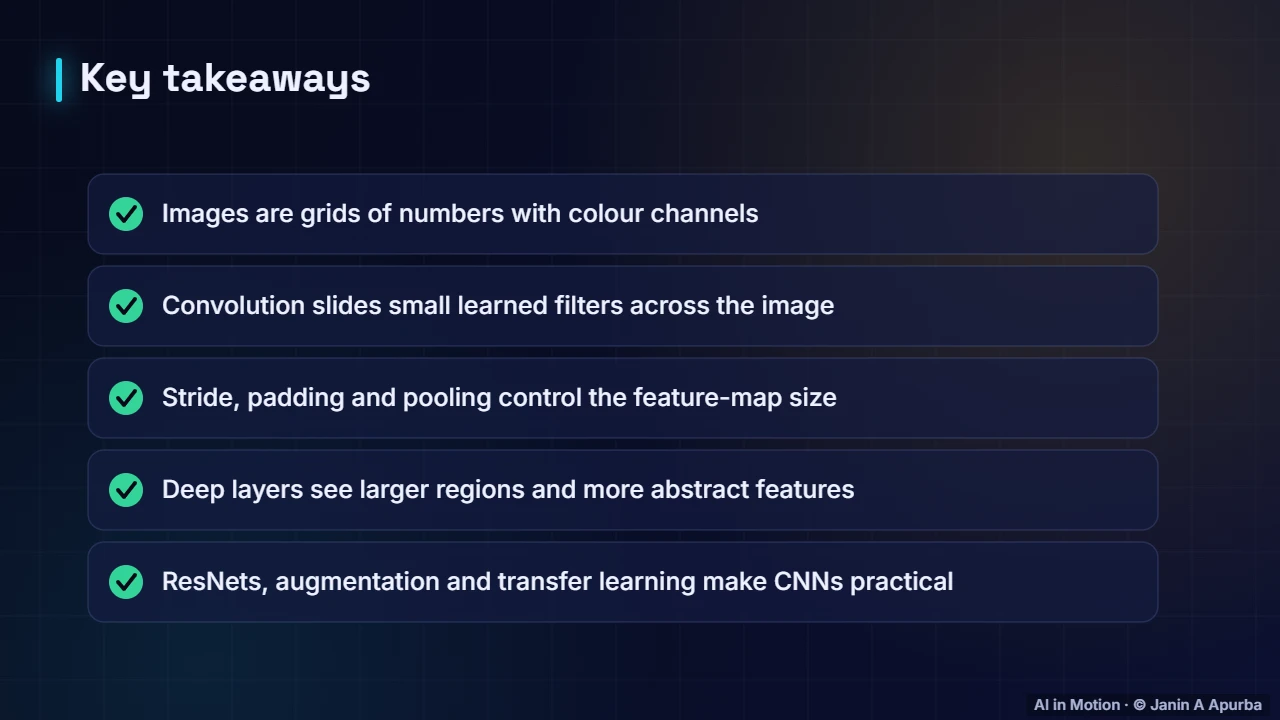
To recap. Images are grids of numbers with colour channels. Convolution slides small learned filters across the image, sharing weights. Stride, padding and pooling control the size of feature maps, and deeper layers see larger regions and more abstract features. Residual connections, augmentation and transfer learning make CNNs practical.
Key takeaways
- An image is a grid of numbers; colour images have three channels (RGB).
- Convolution slides a small kernel across the image, computing a dot product at each position; weights are shared.
- Output size = ⌊(N − K + 2P)/S⌋ + 1; parameters = K × K × C_in × C_out + C_out.
- Pooling shrinks feature maps; stacked layers grow the receptive field and build a feature hierarchy.
- Landmarks: LeNet (1998), AlexNet (2012), VGG/GoogLeNet (2014), ResNet (2015), EfficientNet (2019).
- Batch normalisation, residual connections, data augmentation and transfer learning are standard practice.
Check yourself
- Why do convolutional layers need far fewer parameters than fully connected layers on images?
Show answer
Small filters are shared across all positions — Weight sharing over local patches.
- A 32 × 32 input, 3 × 3 kernel, padding 1, stride 2 gives an output of…
Show answer
16 × 16 — ⌊(32 − 3 + 2)/2⌋ + 1 = 16.
- How many parameters in a 3 × 3 conv from 64 to 128 channels (with biases)?
Show answer
73,856 — 3·3·64·128 + 128.
- What does max pooling keep?
Show answer
The largest value in each window — The strongest activation survives.
- Which idea let ResNet train 152-layer networks?
Show answer
Residual skip connections — Gradients flow through the shortcuts.
Go deeper
- Convolutional Neural Networks: The Core Ideas · The AI Lecture Hall
- Padding, Stride, Pooling and Receptive Fields · The AI Lecture Hall
- LeNet and AlexNet: The Birth of Deep Vision · The AI Lecture Hall
- ResNet in Depth: Architecture, Bottlenecks and Variants · The AI Lecture Hall
- Transfer Learning and Fine-Tuning · The AI Lecture Hall
© 2026 Janin A Apurba, CSE, AUST · Advanced ICT Officer, CNRS-UNHCR. All rights reserved. Notes for the animated lecture at https://ai-in-motion.vercel.app/watch/convolutional-networks-deep-dive.html