Calculus for Machine Learning: Derivatives, Gradients and the Chain Rule — lecture notes
How models learn by following slopes: derivatives, partial derivatives, gradients, gradient descent, saddle points and the chain rule that makes backpropagation possible.
0:001. Introduction
Training a neural network means adjusting millions of numbers so that a loss gets smaller. The only reason this is possible is calculus. In this deep dive we build up derivatives, gradients and the chain rule, and see exactly how they turn into learning.
0:182. Why slopes matter
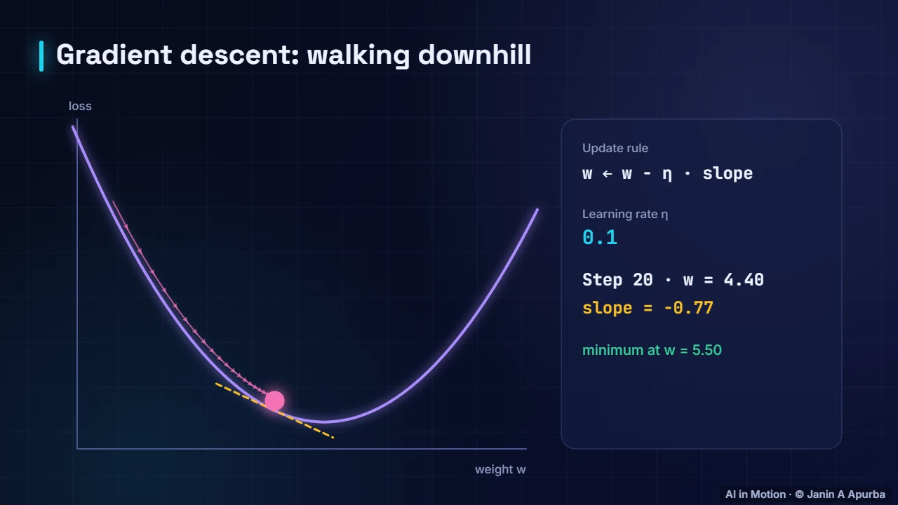
Imagine standing on a hilly loss curve in the fog. You cannot see the lowest point, but you can feel which way the ground slopes under your feet. Take a small step downhill, feel again, and repeat. That is gradient descent, and the slope you feel is the derivative.
0:393. The derivative
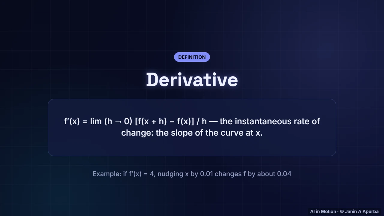
The derivative measures the instantaneous rate of change: how much the output changes for a tiny nudge of the input. Formally, it is the limit of rise over run as the run shrinks to zero. If the derivative is four, a tiny step of point zero one changes the output by about point zero four.
1:024. Secant to tangent
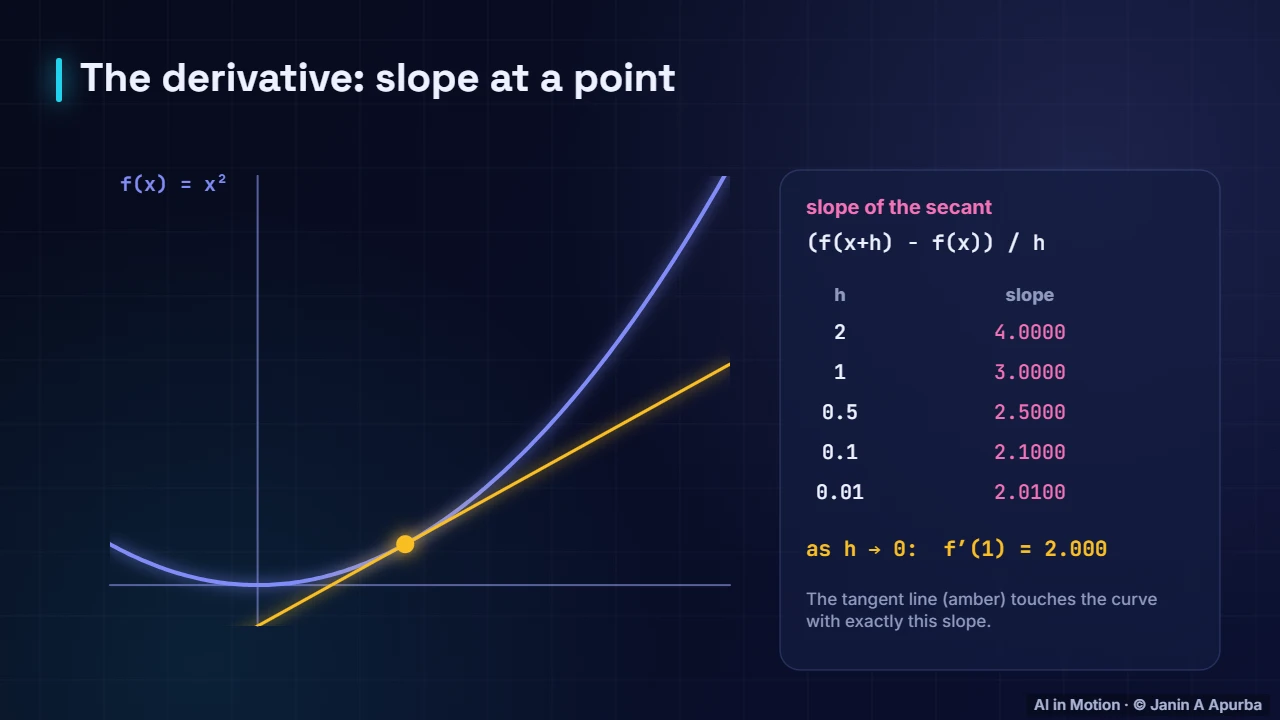
Let us watch the limit happen for f of x equals x squared at x equals one. With a step of two, the secant slope is four. As the step shrinks to one, a half, a tenth and a hundredth, the slope gets closer and closer to two. In the limit we get the tangent line, with slope exactly two.
1:265. Derivative rules
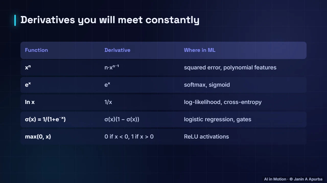
You do not need to derive everything from limits. A handful of rules cover most of machine learning. Powers bring the exponent down. The exponential is its own derivative. The logarithm gives one over x. The sigmoid’s derivative is sigma times one minus sigma, and ReLU’s derivative is zero or one.
1:486. The sigmoid and its slope
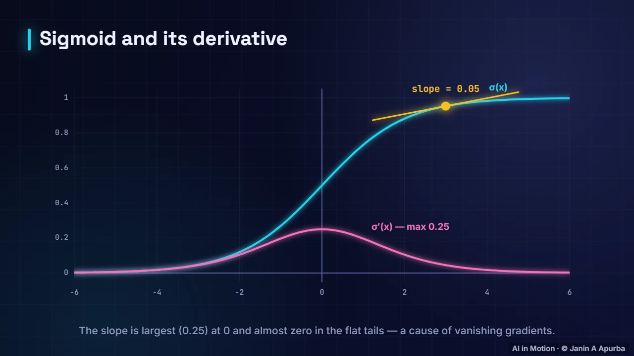
Here is the sigmoid with its derivative in pink. The amber tangent line slides along the curve. The slope is largest at zero, where it equals one quarter, and almost vanishes in the flat tails. This tiny maximum slope is one reason deep networks of sigmoids suffer from vanishing gradients.
2:097. Pause and think
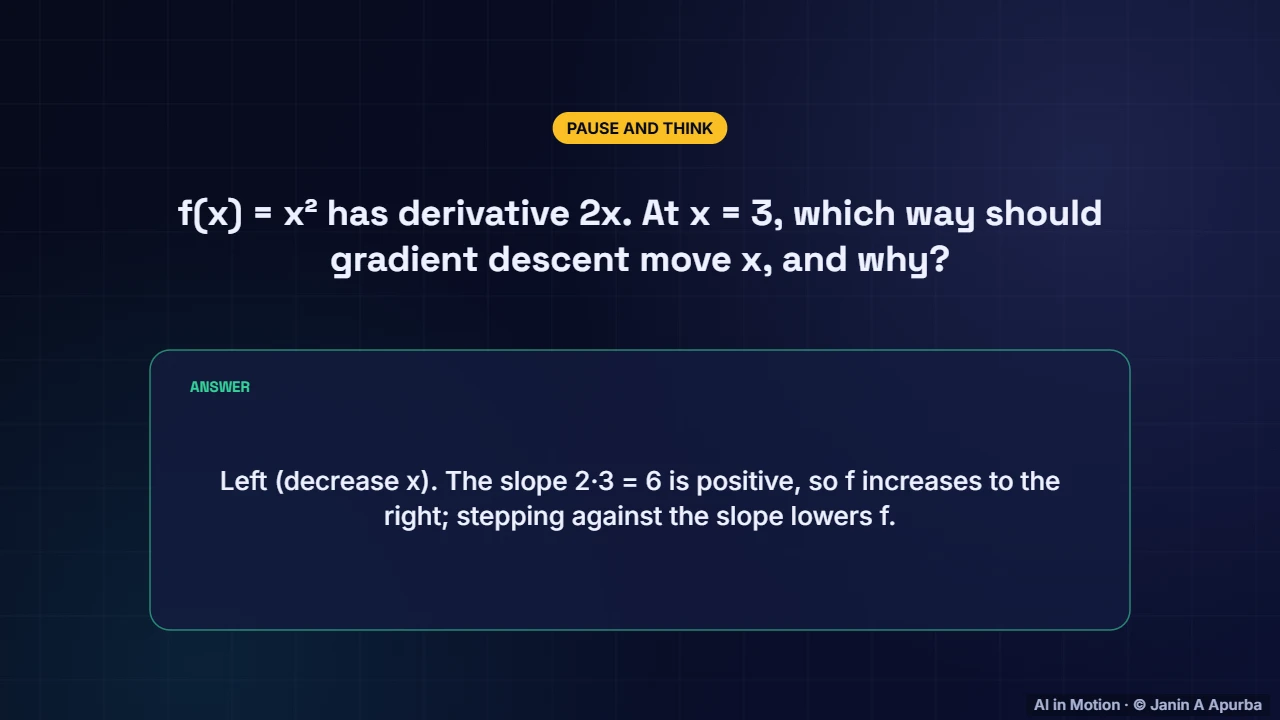
Pause and think. The function x squared has derivative two x. At x equals three, which way should gradient descent move? The slope is six, which is positive, meaning the function rises to the right. So we move left, against the slope, to go downhill.
2:288. Pause and think
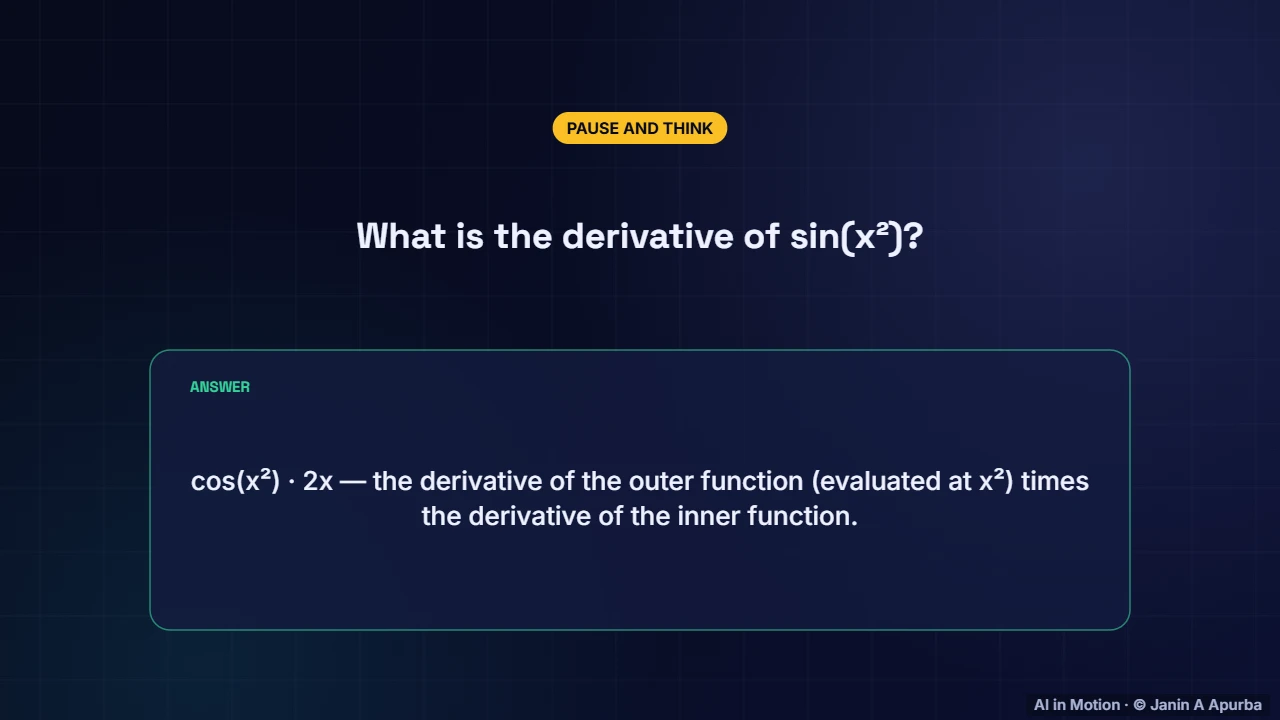
A quick warm up. What is the derivative of the sine of x squared? We will meet the rule formally soon, but have a try. The answer is the cosine of x squared, times two x: the derivative of the outer function, times the derivative of the inner one.
2:499. Partial derivatives
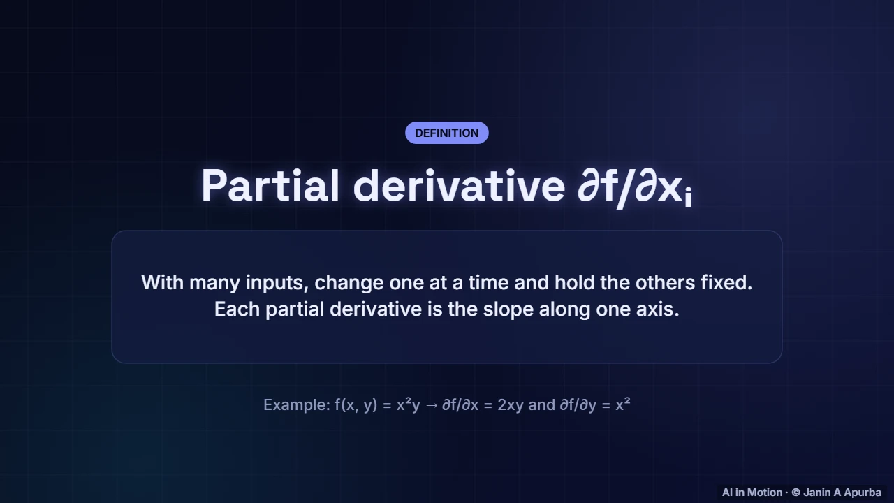
Models have many parameters, not one. A partial derivative measures the slope along one input while all the others are frozen. For x squared times y, the partial derivative with respect to x is two x y, and with respect to y it is x squared.
3:0910. The gradient
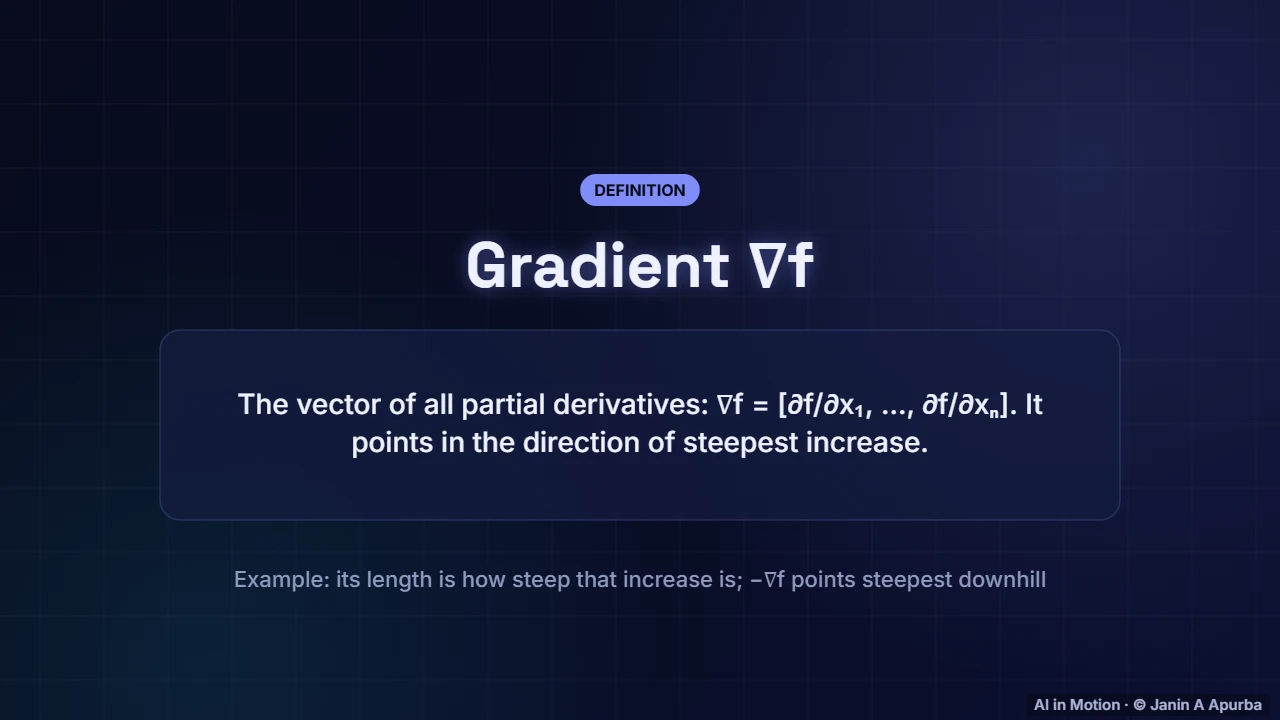
Collect all the partial derivatives into one vector and you have the gradient. The gradient points in the direction of steepest ascent, and its length tells you how steep the climb is. So minus the gradient points straight downhill. For a network, this vector has one entry per parameter.
3:3011. The gradient field
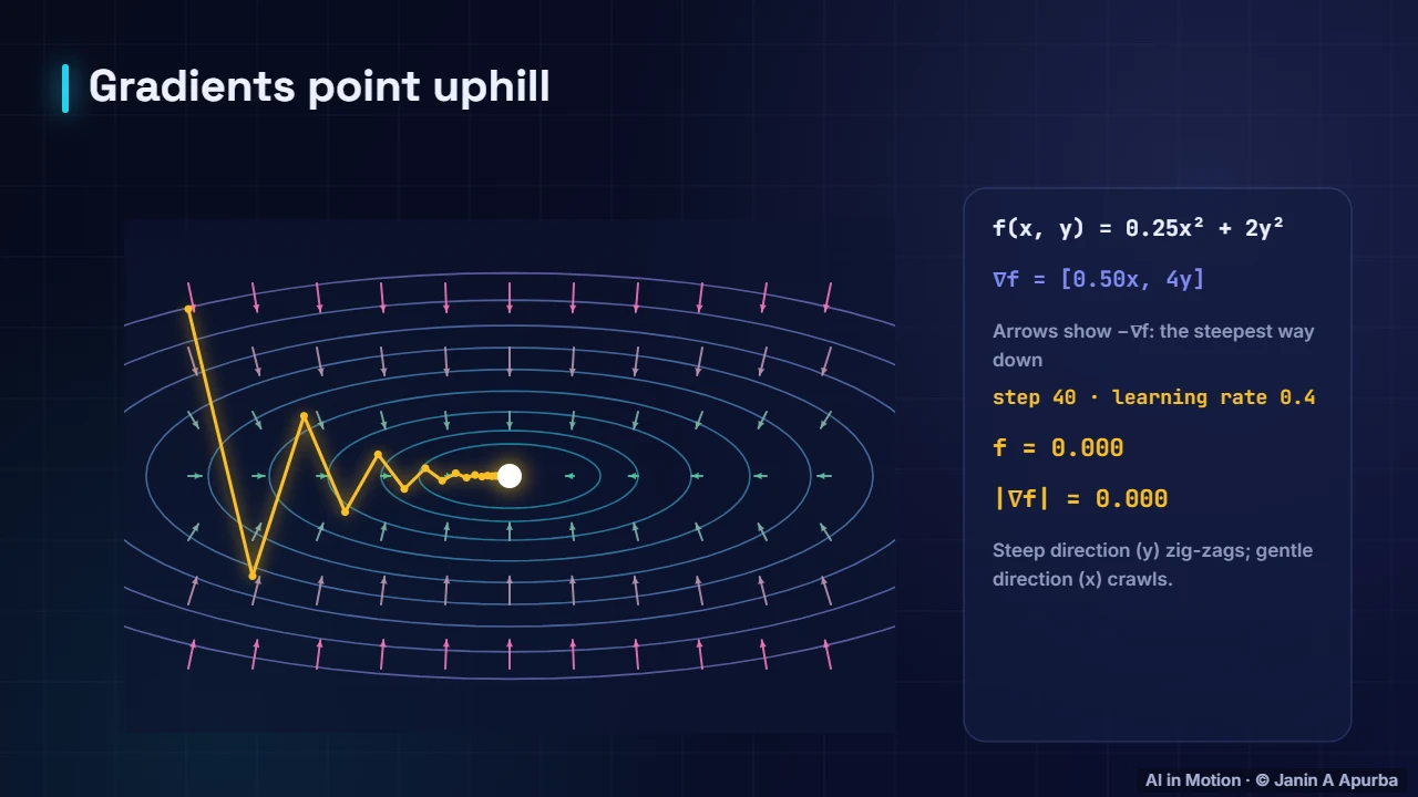
Here is a bowl shaped loss surface drawn as contour lines, with arrows showing minus the gradient at many points. The ball follows the arrows downhill. Notice how it zig zags across the steep direction while crawling along the gentle one. That shape comes from very different curvatures along the two axes.
3:5212. The update rule
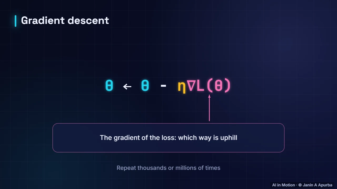
The update rule is simple. Every parameter moves a small step against the gradient of the loss, scaled by the learning rate, eta. Repeat thousands or millions of times. Every modern optimiser, including momentum and Adam, is a refinement of this one line.
4:1013. Learning rate too small
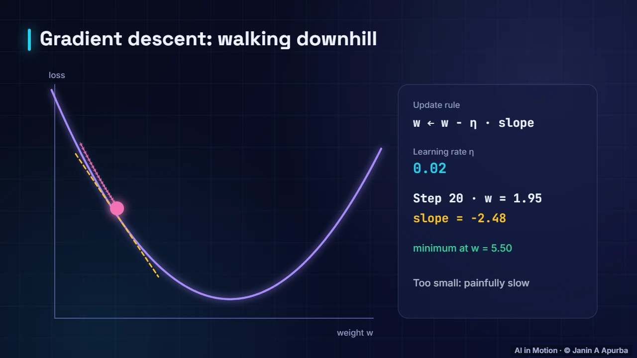
The learning rate matters enormously. With a tiny learning rate, each step is safe but minuscule. After twenty steps we have barely moved, and training would take forever. Models trained this way waste time and compute.
4:2614. Learning rate too large
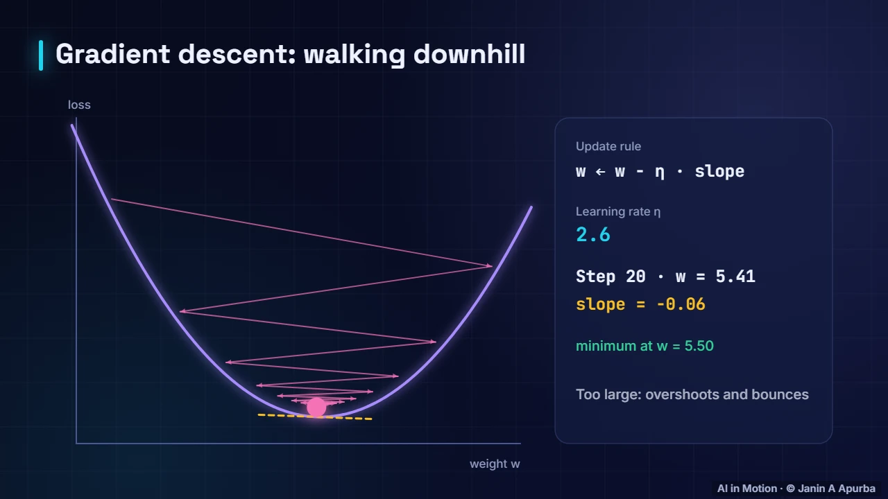
With a learning rate that is too large, each step overshoots the minimum and lands on the other side of the valley. The point bounces back and forth, and if the rate is larger still, the loss can explode entirely. Finding a good learning rate is one of the first jobs when training a model.
4:4915. Curvature
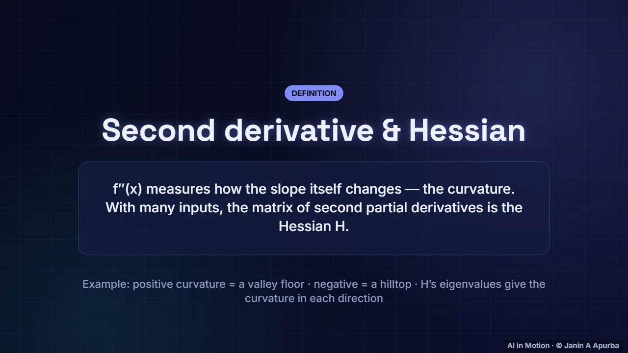
The second derivative measures how the slope itself changes: the curvature. Positive curvature means a valley, and negative curvature means a hilltop. With many parameters, the second derivatives form the Hessian matrix, and its eigenvalues describe the curvature along each direction of the loss surface.
5:0816. Convexity
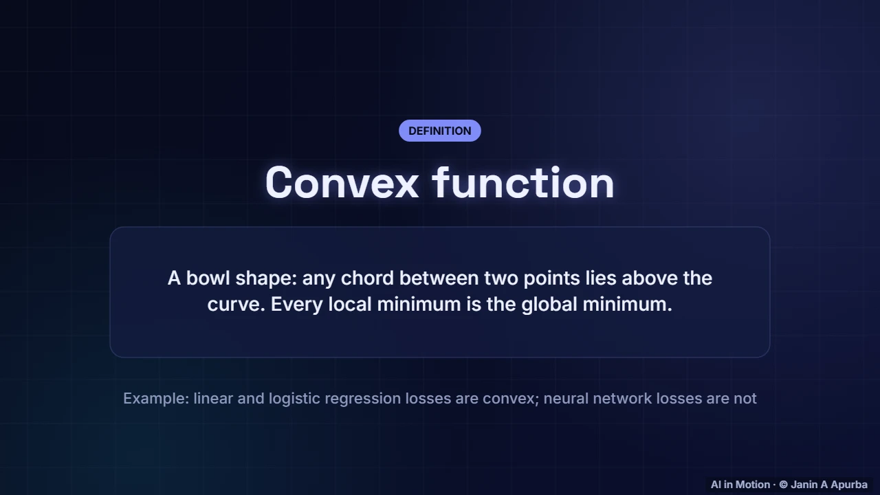
Some functions are convex, shaped like a bowl, so that any line segment between two points on the curve lies above it. For convex functions, every local minimum is the global minimum, and gradient descent is guaranteed to find it. Linear and logistic regression have convex losses.
5:2817. Non-convex landscapes
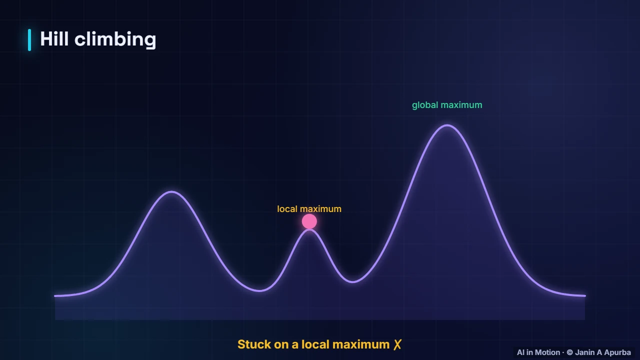
Neural network losses are not convex. Their landscapes have many valleys, ridges and plateaus. Here a simple hill climber gets stuck on a local peak. Surprisingly, in very high dimensions, true bad local minima are rarer than people once feared, and the bigger obstacles are flat regions and saddle points.
5:4918. Saddle points
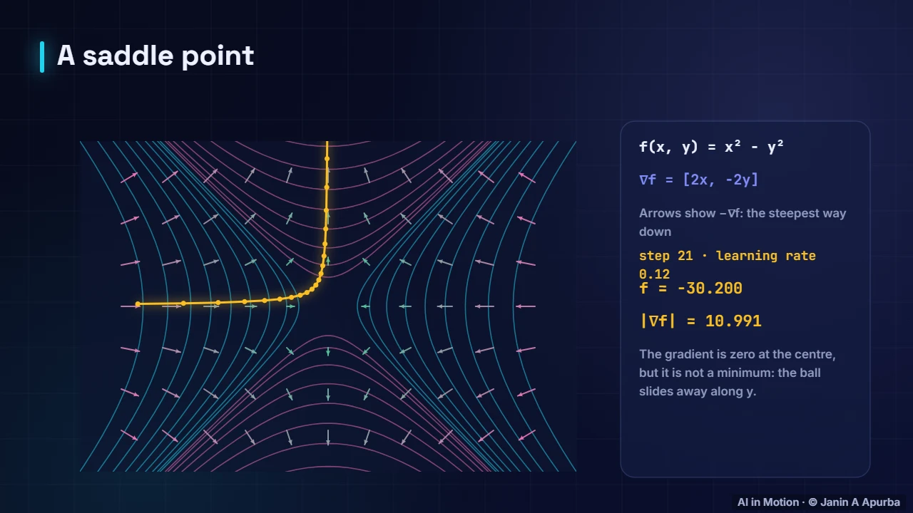
This is a saddle point: the surface curves up in one direction and down in another, like a horse’s saddle. The gradient is exactly zero at the centre, yet it is not a minimum. The ball starting almost on the ridge eventually slides away. In high dimensions, most critical points are saddles.
6:1119. Pause and think

Pause and think. At some point the gradient is exactly zero. Are you guaranteed to be at a minimum? No. A zero gradient could mean a minimum, a maximum or a saddle point. To tell them apart you need the curvature, which is measured by second derivatives, collected in the Hessian matrix.
6:3320. Better optimisers
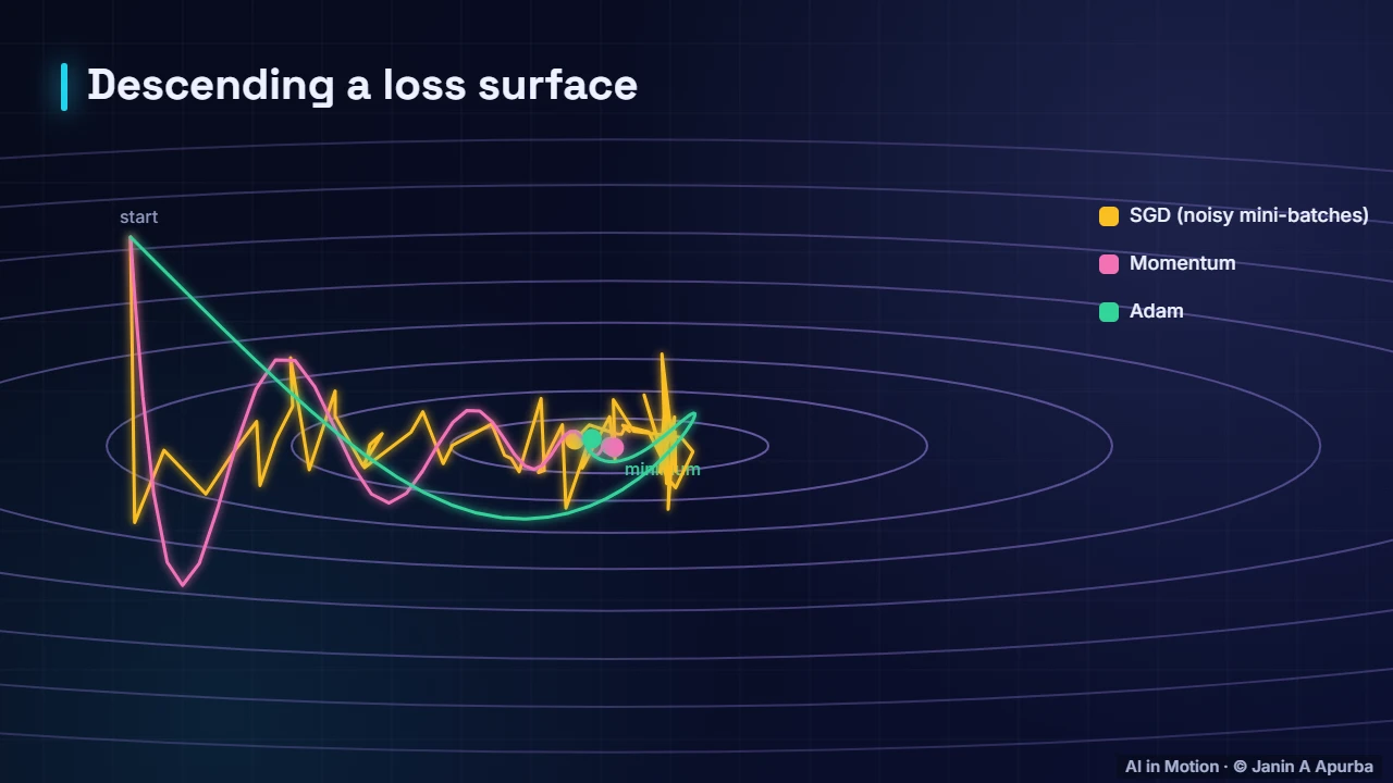
Better optimisers use extra tricks. Momentum accumulates a running average of past gradients, so it keeps moving through flat regions and damps the zig zag. Adam also adapts the step size for each parameter separately. On this surface you can see them take very different paths.
6:5321. The chain rule
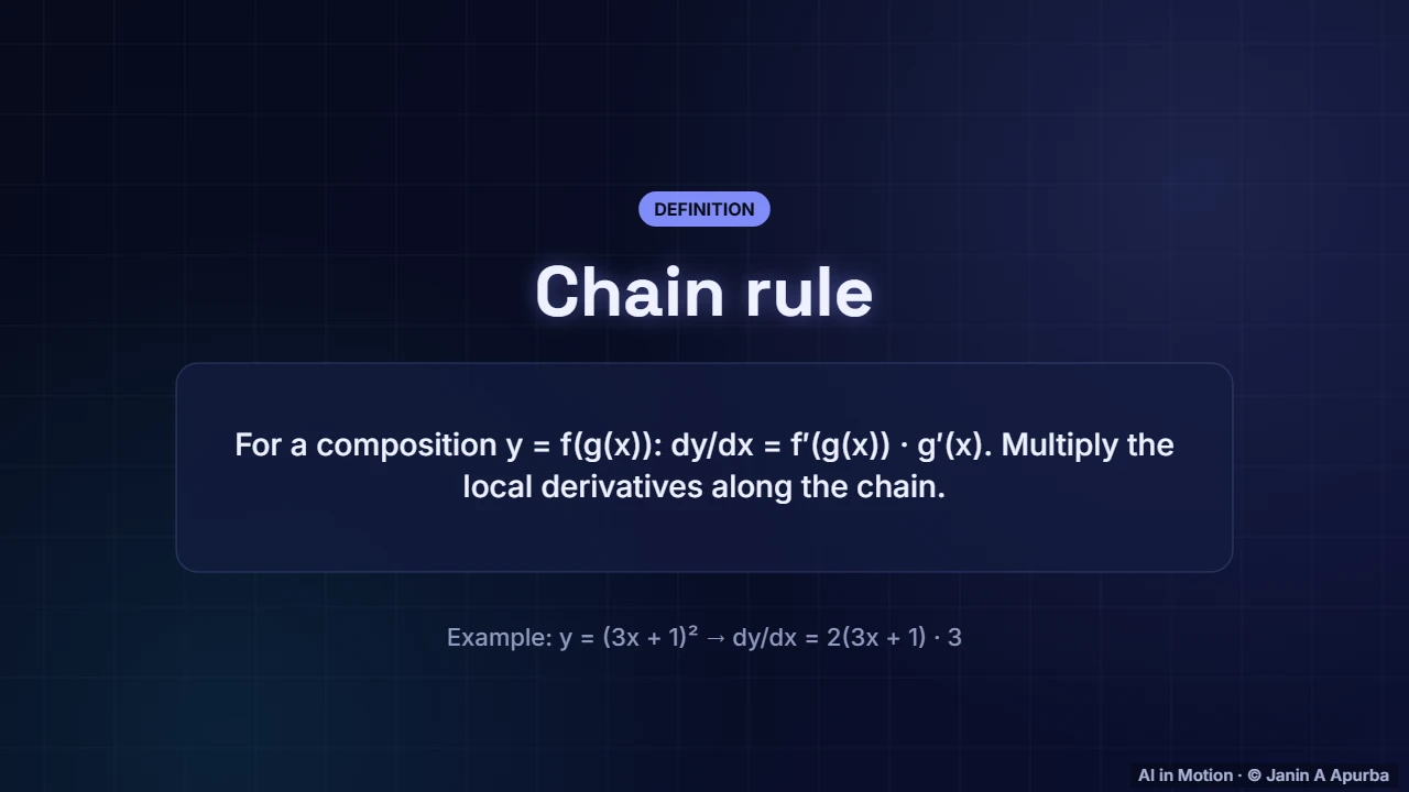
Now the most important rule for deep learning: the chain rule. When functions are nested, one inside another, the derivative of the whole is the product of the local derivatives along the chain. For three x plus one, squared, the derivative is two times three x plus one, times three.
7:1422. Forward and backward
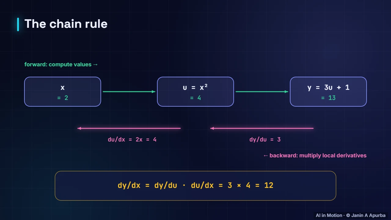
Here is the chain rule as a pipeline. The forward pass computes values: x is two, u is four, and y is thirteen. The backward pass multiplies local derivatives from right to left: three times four gives twelve. Change x by a tiny amount, and y changes twelve times as much.
7:3623. Jacobians
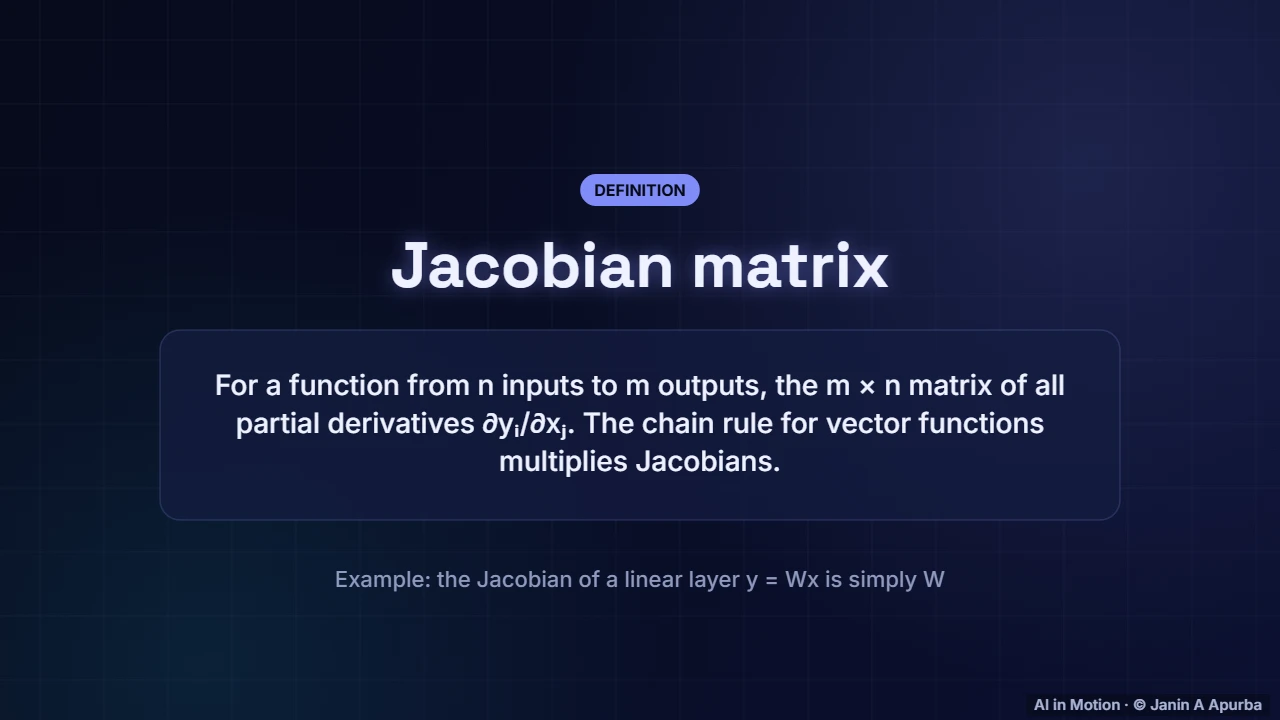
When a function maps many inputs to many outputs, its derivatives form a matrix called the Jacobian. The chain rule for vector functions multiplies Jacobians together. For a linear layer the Jacobian is just the weight matrix, which is why backpropagation is full of transposed weight matrices.
7:5624. Backpropagation
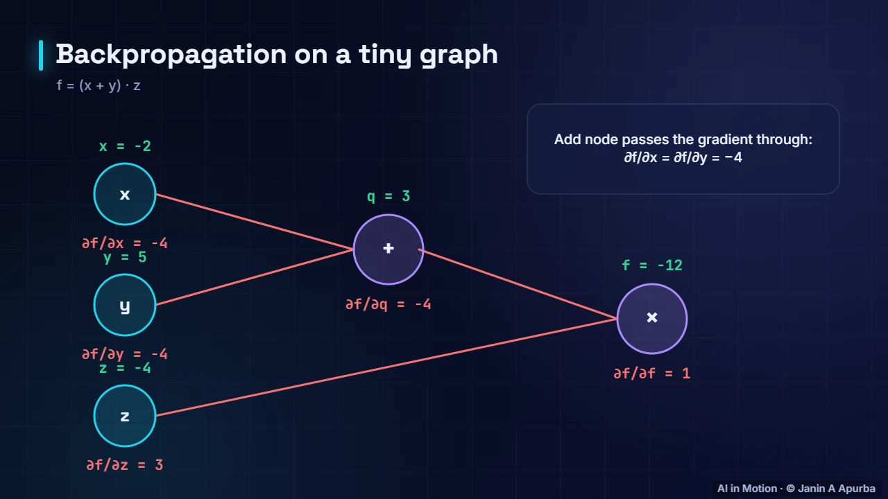
Backpropagation is simply the chain rule applied systematically to a computational graph. The forward pass stores every intermediate value. The backward pass starts from the loss and multiplies local derivatives node by node, delivering the gradient for every parameter in one sweep.
8:1425. Why backprop wins
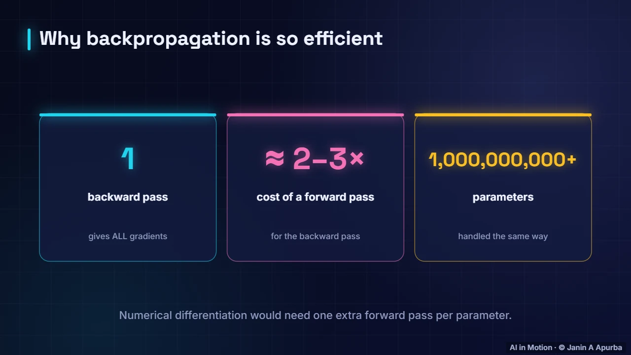
Backpropagation is remarkably efficient. A single backward pass, costing roughly two to three forward passes, delivers the gradient for every parameter at once, whether there are a thousand or a billion. Estimating gradients by nudging each parameter separately would need one extra pass per parameter.
8:3326. Vanishing gradients
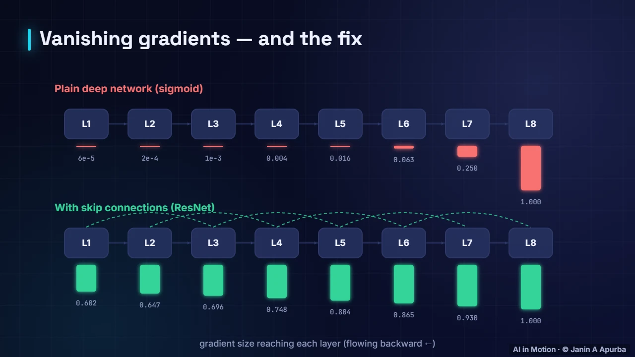
The chain rule also explains a classic problem. In a deep network the gradient is a long product of local derivatives. If those are mostly below one, as with sigmoids, the product shrinks towards zero and early layers stop learning. Skip connections, as in ResNet, give the gradient a shortcut.
8:5427. Activations and their slopes
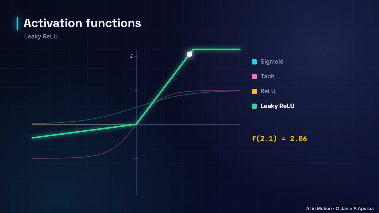
The choice of activation function matters because of these slopes. Sigmoid and tanh flatten out for large inputs, so their derivatives vanish there. ReLU has a slope of exactly one for positive inputs, which lets gradients pass through many layers, one reason it made very deep networks trainable.
9:1528. Autodiff in PyTorch
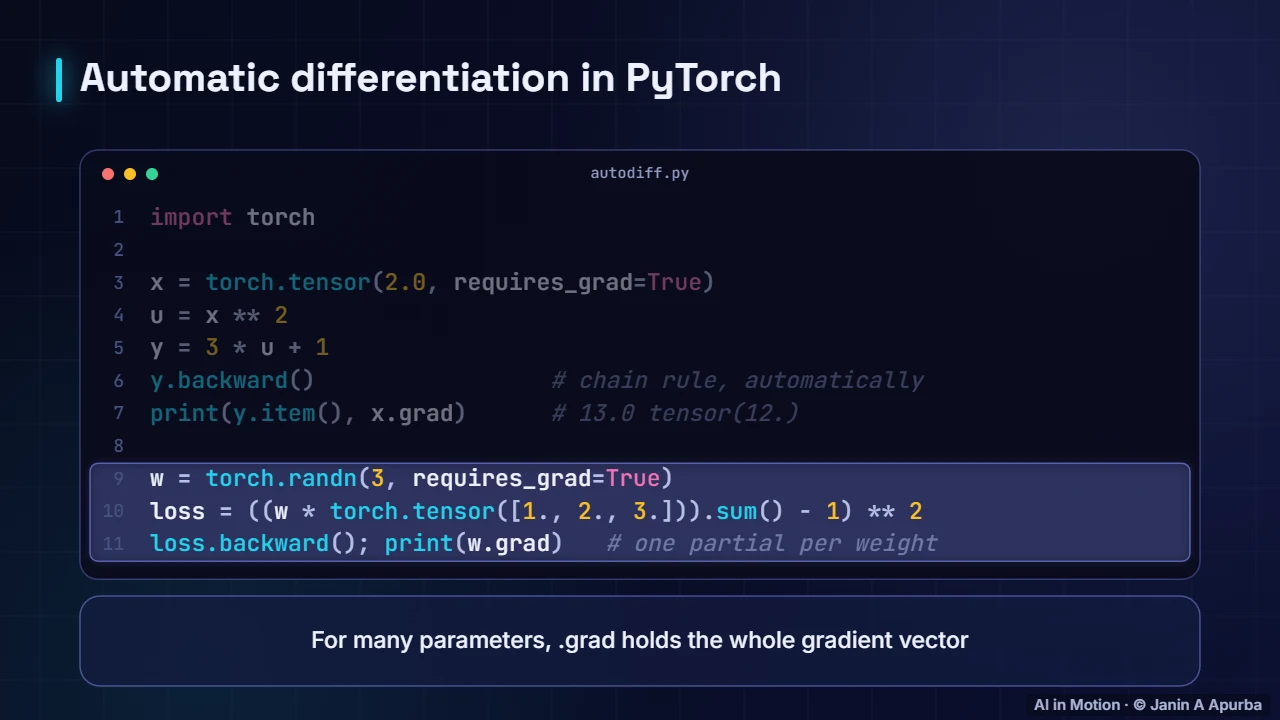
In practice nobody differentiates by hand. Frameworks like PyTorch record the forward computation and apply the chain rule automatically. Here the same chain gives y equals thirteen and a gradient of twelve. With a vector of weights, the grad attribute holds one partial derivative per weight.
9:3529. The training loop
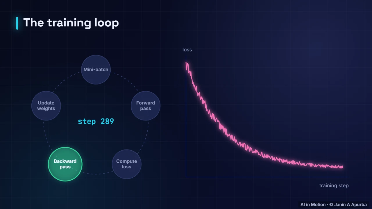
Put it all together and you have the training loop. Take a batch of data, run the forward pass, compute the loss, run backpropagation to get the gradient, and let the optimiser take a step. Repeat. Every model you have heard of, from spam filters to GPT, is trained this way.
9:5630. Pause and think

A practical question. Your training loss suddenly becomes not a number after a few hundred steps. What should you check? Most often it is exploding gradients, so lower the learning rate or clip gradients, or a numerically unstable operation such as the log of zero or the exponential of a huge number.
10:1831. Practical tips
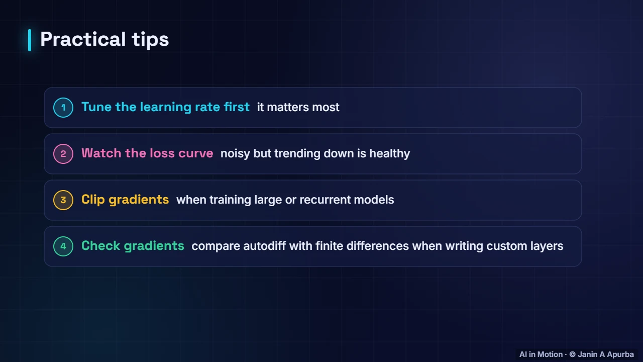
Some practical tips. Tune the learning rate first, because it matters more than almost anything else. Watch the loss curve. Clip gradients for large or recurrent models. And when you write a custom layer, check its gradients against small finite differences.
10:3632. Recap
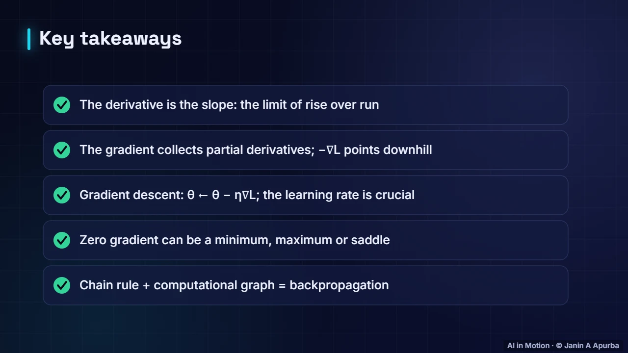
To recap. The derivative is the slope, a limit of rise over run. The gradient collects all the partial derivatives, and minus the gradient points downhill. Gradient descent steps against it, with the learning rate setting the size. A zero gradient may be a saddle, and the chain rule applied to a graph is backpropagation.
Key takeaways
- A derivative is the limit of rise over run: the slope at a point.
- The gradient ∇f is the vector of partial derivatives and points in the direction of steepest increase.
- Gradient descent updates θ ← θ − η∇L; too small a learning rate is slow, too large diverges.
- Convex losses have a single global minimum; neural-network losses are non-convex with many saddle points.
- The chain rule multiplies local derivatives; backpropagation applies it to a whole computational graph.
- Frameworks such as PyTorch compute gradients automatically (autodiff).
Check yourself
- What is the derivative of x² at x = 1?
Show answer
2 — d/dx x² = 2x = 2.
- Which direction does −∇L point?
Show answer
Steepest decrease of the loss — The gradient points uphill; its negative points downhill.
- What is the largest value of the sigmoid’s derivative?
Show answer
0.25 — σ′(0) = 0.5 × 0.5 = 0.25.
- If y = 3u + 1 and u = x², what is dy/dx at x = 2?
Show answer
12 — dy/du · du/dx = 3 × 2x = 3 × 4 = 12.
- A point with zero gradient that curves up one way and down another is a…
Show answer
Saddle point — Mixed curvature defines a saddle.
Go deeper
- Derivatives, Gradients and the Chain Rule · The AI Lecture Hall
- Gradient Descent: Theory, Step Sizes and Convergence · The AI Lecture Hall
- Backpropagation Derived Step by Step · The AI Lecture Hall
© 2026 Janin A Apurba, CSE, AUST · Advanced ICT Officer, CNRS-UNHCR. All rights reserved. Notes for the animated lecture at https://ai-in-motion.vercel.app/watch/calculus-for-machine-learning.html